Fear and Greed is Shifting and Models Don’t Avoid the Feelings

October 27, 2015 By Mike Shell in Absolute Return, Active Risk Management, Back Testing, Fear and Greed Index, Hiring a Portfolio Manager, Investor Behavior Modification, Investor Sentiment, tactical risk management, U.S. Stock Market Leave a comment

Investors are driven by fear and greed. That same fear and greed drives market prices. It’s Economics 101 “Supply and Demand”. Greed drives demand, fear drives selling pressure. In fact, investors are driven by the fear of losing more money when their account is falling and fear missing out if they have cash when markets go up. Most investors tend to experience a stronger feeling from losing money than they do missing out. Some of the most emotional investors oscillate between the fear of missing out and the fear of losing money. These investors have to modify their behavior to avoid making mistakes. Quantitive rules-based systematic models don’t remove the emotion.

Amateur portfolio managers who lack experience sometimes claim things like: “our quantitive rules-based systematic models removes the emotion”. That couldn’t be further from the truth. Those who believe that will eventually find themselves experiencing feelings from their signals they’ve never felt before. I believe it’s a sign of high expectations and those expectations often lead to even stronger reactions. It seems it’s the portfolio managers with very little actual performance beyond a backtest that make these statements. They must believe a backtested model will act to medicate their feelings, but it doesn’t actually work that way. I believe these are the very people who over optimize a backtest to make it perfectly fit historical data. We call it “curve-fitting” or “over-fitting”, but it’s always “data mining”. When we backtest systems to see how they would have acted in the past, it’s always mining the data retroactively with perfect hindsight. I’ve never had anyone show me a bad backtest. If someone backtests entry and exit signals intended to be sold as a managed portfolio you can probably see how they may be motivated to show the one that is most optimized to past data. But, what if the future is very different? When it doesn’t work out so perfectly, I think they’ll experience the very feelings they wish to avoid. I thought I would point this out, since many global markets have been swinging up and down. I’m guessing some may be feeling their feelings.

The CNN Fear & Greed Index shows investor fear and greed shifted to Extreme Fear a month ago as the popular U.S. stock indexes dropped about -12% or more. Many sectors and other markets were worse. Since then, as prices have been trending back up, Greed is now the driver again. I believe fear and greed both drives market prices but also follows price trends. As prices move lower and lower, investors who are losing money get more and more afraid of losing more. As prices move higher and higher, investors get more and more greedy. If they have reduced exposure to avoid loss, they may fear missing out.

Source: http://money.cnn.com/data/fear-and-greed/

This is the challenge in bear markets. In a bear market, market prices swing up and down along the way. It’s these swings that lead to mistakes. Below is a chart of how the Fear and Greed Index oscillates to high and low points over time. Investors who experience these extremes in emotion have the most trouble and need to modify their behavior so they feel the right feeling at the right time. Or, hire a manager with a real track record who can do it for them and go do something more enjoyable.

Source: http://money.cnn.com/data/fear-and-greed/

The Trend of the U.S. Stock Market

September 9, 2015 By Mike Shell in Absolute Return, Actively Manage Risk, Global Directional Trends, risk managed, S&P 500, tactical risk management, U.S. Stock Market Leave a comment

When I say “The Trend” that could mean an infinite number of “trends“. The general definition of “trend” is a general tendency or course of events.

But when I speak of “The Trend” I mean a direction that something is moving, developing, evolving, or changing. A trend, to me, is a directional drift, one way or another. When I speak of price trends, I mean the directional drift of a price trend that can be up, down, or sideways.

Many investors are probably wondering about the current trend of the U.S. stock market. So, I will share a quick observation since one of the most popular U.S. stock indexes seems to be right at a potential turning point.

Below is a 6 month price chart of the S&P 500 stock index. The S&P 500® is widely regarded as a gauge of large-cap U.S. equities. Clearly, prior to late August the stock index was drifting sideways. It was oscillating up and down in a range of 3% to 4% swings, but overall it wasn’t making material higher highs or lower lows. That is, until late August when it dropped about -12% below its prior high. Now, we see with today’s action the stock index is attempting reach or breach it’s very recent peak reached on August 27th. If the index moves above this level, we may consider it a short-term uptrend. We can already observe the index has made a higher low.

Source: Shell Capital Management, LLC created with http://www.stockcharts.com

You can probably see how the next swing will determine the direction of the trend. If it breaks to the upside, it will be an uptrend as defined by “higher highs and higher lows”. Although, that is a very short-term trend, since it will happen within a more intermediate downtrend.

My point is to observe how trends drift and unfold over time, not to predict which way they will go, but instead to understand and define the direction of “the trend”. And, there are many different time frames we can consider.

If this trend keeps going up, supply and demand will determine for how long and how far. If it keeps drifting up, I would expect it may keep going up until some inertia changes it. Inertia is the resistance to change, including a resistance to change in direction.

But if it instead goes back down to a new low, I bet we’ll see some panic selling driving it even lower.

The real challenge of directional price trends is if this is the early stage of a larger downward trend (like a bear market), there will be many swings along the way. In the last bear market, there were 13 swings that ranged from 10% to 27% as this stock index took about 18 months to decline -56%.

Below is the same stock index charted with a percentage chart to better show the percent changes over the past 6 months. You can probably see how it gives a little different perspective.

Source: Shell Capital Management, LLC created with http://www.stockcharts.com

I don’t necessarily make my tactical decisions based on any of this. I enjoy watching it all unfold and I necessarily need to define the trend and understand it as it all plays out. I want to know what the direction of the trend is based on my time frame, and know when that changes.

I believe world markets require active risk management and defining directional trends. For me, that means predefining my risk in advance in each position and across the portfolio.

______

For informational and educational purposes only, not a recommendation to buy or sell and security, fund, or strategy. Past performance and does not guarantee future results. The S&P 500 index is an unmanaged index and cannot be invested into directly. Please visit this link for important disclosures, terms, and conditions.

Using the Month of September to Understand Probability and Expectation

September 1, 2015 By Mike Shell in Absolute Return, Adapting to Change, Asymmetric Observation, Asymmetric Payoff, Asymmetric Risk, Asymmetric Risk Reward, Critical Thinking, Independent Thinking, Mathematical Expectation, Probability Leave a comment

September is the month when the U.S. stock market’s three most popular indexes usually perform the poorest. So say the headlines every September.

I first wrote this in September 2013 after many commentators had published information about the seasonality of the month of September. Seasonality is the historical tendency for certain calendar periods to gain or lose value. However, when commentators speak of such probabilities, they rarely provide a clear probability and almost never the full mathematical expectation. Without the mathematical expectation, probability alone is of little value or no value. I’ll explain why.

For those of us focused on actual directional price trends it may seem a little silly to discuss the historical probability of gain or loss for a single month. However, even though I wouldn’t make decisions based on it, we can use the seasonal theme to explain the critical importance of both probability and mathematical expectation.

“From 1928-2012 the S&P 500 was up 39 months and down 46 months in September. It is down 55% of the time in September…”

“Dow Jones Industrial Average 1886-2004 (116 years) 49 years the Dow was up in September, in 67 years the Dow was down in September. It’s down 58% of the time in September…”

Those are probability statements. But they say nothing about how much it was up or down.

First, let’s define probability.

Probability is likelihood. It is a measure or estimation of how likely it is that something will happen or that a statement is true. Probabilities are given a range of value between 0% chance (it will not happen) and 100% chance (it will happen). There are few things so certain as 0% and 100%, so most probabilities fall in between. The higher the degree of probability, the more likely the event is to happen, or, in a longer series of samples, the greater the number of times such event is expected to happen.

But that says nothing about how to calculate probability and apply it. One thing to realize about probability is that it is the math for dealing with uncertainty. When we don’t know an outcome, it is uncertain. It is probabilistic, not a sure thing. Probability provides us our best estimation of the outcome.

As I see it, there are two ways to calculate probability: subjectively and objectively.

Subjective Probability: assigns a likelihood based on opinions and confidence (degree of belief) in those opinions. It may include “expert” knowledge as well as experimental data. For example, the majority of the research and news is based on “expert opinion”. They may state their belief and then assign a probability: “I believe the stock market has a X% chance of going down.” They may go on to add a good sounding story to support their hypothesis. You may see how that is subjective.

Objective Probability: assigns a likelihood based on numbers. Objective probability is data-driven. The popular method is frequentist probability: the probability of a random event means the relative frequency of occurrence of an experiment’s outcome when the experiment is repeated. This method believes probability is the relative frequency of outcomes over the long run. We can think of it as the historical tendency of the outcome. For example, if we flip a fair coin, its probability of landing on heads is 50% and tails is 50%. If we flip it 10 times, it could land on heads 7 and tails 3. That outcome implies 70%/30%. To prove the coin is “fair” (balanced on both sides), we would need to flip it more times to get a large enough sample size to realize the full probability. If we flip it 30 times or more it is likely to get closer and closer to 50%/50%. The more frequency, the closer it gets to its probability. You may see see why I say this is more objective: it’s based on actual historical data.

If you are a math person and logical thinker, you may get this. I have a hunch many people don’t like math, so they’d rather hear a good story. Rather than checking the stats on a game, they’d rather hear some guru’s opinion about who will win.

Which has more predictive power? An expert opinion or the fact that historically the month of September has been down more often than it’s up? Predictive ability needs to be quantified by math to determine if it exists and opinions are often far too subjective to do that. We can do the math based on historical data and determine if it is probable, or not.

As I said in September is statistically the worst month for the stock market the data shows it is indeed statistically significant and does indeed have predictive ability, but not necessarily enough to act on it. Instead, I suggest it be used to set expectations of what may happen: the month of September has historically been the worst performance month for the stock indexes. So, we shouldn’t be surprised if it ends in the red. It’s that simple.

Theory-driven researchers want a cause and effect story to go with their beliefs. If they can’t figure out a good reason behind the phenomenon, they may reject it even though the data is what it is. One person commented to me that he didn’t believe the September data has predictive value, even though it does, and he provided nothing to disprove it. Probabilities do need to make sense. Correlations can occur randomly, so logical reasoning behind the numbers may be useful. For example, one theory for a losing September is it is the fiscal year end of many mutual funds and fund managers typically sell losing positions before year end to realize losses to offset gains.

I previously stated a few different probabilities about September: what percentage of time the month is down. In September is statistically the worst month for the stock market I didn’t mention the percent of time the month is negative, only that on average it’s down X% since Y. It occurred to me that most people don’t seem to understand probability and more importantly, the more complete equation of expectation.

Expectation

There are many different ways to define expectation. We may initially think of it as “what we expect to happen”. In many ways, it’s best not to have expectations about the future. Our expectations may not play out as we’d hoped. If we base our investment decisions on opinion and expectations don’t pan out, we may stick with our opinion anyway and eventually lose money. The expectation I’m talking about is the kind that I apply: mathematical expectation.

So far, we have determined probability of September based on how many months it’s down or up. However, probability alone isn’t enough information to make a logical decision. First of all, going back to 1950 using the S&P 500 stock index, the month of September is down about 53% of the time and ends the month positive about 47% of the time. That alone isn’t a huge difference, but what makes it more meaningful is the expectation. When it’s down 53% of the time, it’s down -3.8% and when it’s up 47% of the time it’s up an average of 3.3%. That results in an expected value of -0.50% for the month of September. If we go back further to 1928, which includes the Great Depression, it’s about -1.12%.

The bottom line is the math says “based on historical data, September has been the worst month for the stock market”. We could then say “it can be expected to be”. But as I said before, it may not be! And, another point I have made is the use of multiple time frames for looking at the data, which is a reminder that by intention: probability is not exact. It can’t be, it’s not supposed to be, and doesn’t need to be! Probability and expectation are the maths of uncertainty. We don’t know in advance many outcomes in life, but we can estimate them mathematically and that provides a sound logic and a mathematical basis for believing what we do.

We’ve made a whole lot of the month of September, but I think it made for a good opportunity to explain probability and expectation that are the essence of portfolio management. It doesn’t matter so much how often we are right or wrong, but instead the probability and the magnitude. Asymmetric returns are created by more profit, less loss. Mathematical expectation provides us a mathematical basis for believing a method works, or not. Not knowing the future; it’s the best we have.

Rather than seasonal tendencies, I prefer to focus on the actual direction of global price trends and directly manage the risk in individual my positions.

Subscribe to Blog via Email

Connect with me on Linkedin and Follow me on Twitter.

Why Index ETFs Over Individual Stocks?

August 8, 2015 By Mike Shell in Absolute Return, Actively Manage Risk, Adapting to Change, Alternative Investment, Asymmetric Observation, Asymmetric Payoff, Asymmetric Risk, Asymmetric Risk Reward, Asymmetric Sector Exposure, Empirical Observation, ETF Strategist, Global Asset Allocation, Global Directional Trends, Managed Momentum, Managed Volatility, Momentum Relative Strength, Sector ETF, Sector Rotation, Sector Trends, Tactical Asset Allocation, Tactical ETF Portfolio Management, Trend Following Leave a comment

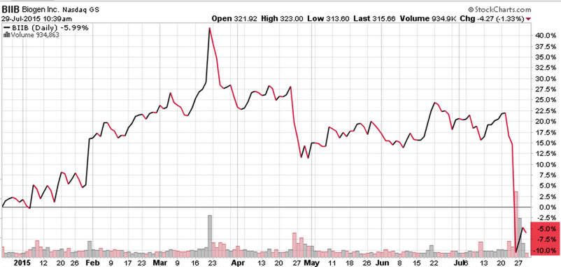
A fellow portfolio manager I know was telling me about a sharp price drop in one of his positions that was enough to wipe out the 40% gain he had in the stock. Of course, he had previously told me he had a quick 40% gain in the stock, too. That may have been his signal to sell. Biogen, Inc (BIIB) recently declined about -30% in about three days. Easy come, easy go. Below is a price chart over the past year.

Source: Shell Capital Management, LLC created with http://www.stockcharts.com

Occasionally investors or advisors will ask: “Why trade index ETFs instead of individual stocks?“. An exchange-traded fund (ETF) is an investment fund traded on stock exchanges, much like stocks. Until ETFs came along the past decade or so, gaining exposure to sectors, countries, bond markets, commodities, and currencies wasn’t so easy. It has taken some time for portfolio managers to adapt to using them, but ETFs are easily tradable on an exchange like stocks. Prior to ETFs, those few of us who applied “Sector Rotation” or “Asset Class Rotation” or any kind of tactical shifts between markets did so with much more expensive mutual funds. ETFs have provided us with low cost, transparent, and tax efficient exposure to a very global universe of stocks, bonds, commodities, currencies, and even alternatives like REITs, private equity, MLP’s, volatility, or inverse (short). Prior to ETFs we would have had to get these exposures with futures or options. I saw the potential of ETFs early, so I developed risk management and trend systems that I’ve applied to ETFs that I would have previously applied to futures.

On the one hand, someone who thinks they are a good stock picker are enticed to want to get more granular into a sector and find what they believe is the “best” stock. In some ways, that seems to make sense if we can weed out the bad ones and only hold the good ones. It really isn’t so simple. I view everything a reward/risk ratio, which I call asymmetric payoffs. There is a tradeoff between the reward/risk of getting more detailed and focused in the exposure vs. having at least some diversification, such as exposure to the whole sector instead of just the stock.

Market Risk, Sector Risk, and Stock Risk

In the big picture, we can break exposures into three simple risks (and those risks can be explored with even more detail). We’ll start with the broad risk and get more detailed. Academic theories break down the risk between “market risk” that can’t be diversified away and “single stock” and sector risk that may be diversified away.

Market Risk: In finance and economics, systematic risk (in economics often called aggregate risk or undiversifiable risk) is vulnerable to events which affect aggregate outcomes such as broad market declines, total economy-wide resource holdings, or aggregate income. Market risk is the risk that comes from the whole market itself. For example, when the stock market index falls -10% most stocks have declined more or less.

Stock and Sector Risk: Unsystematic risk, also known as “specific risk,” “diversifiable risk“, is the type of uncertainty that comes with the company or industry itself. Unsystematic risk can be reduced through diversification. If we hold an index of 50 Biotech stocks in an index ETF its potential and magnitude of a large gap down in price is less than an individual stock.

You can probably see how holding a single stock like Biogen has its own individual risks as a single company such as its own earnings reports, results of its drug trials, etc. A biotech stock is especially interesting to use as an example because investing in biotechnology comes with a unique host of risks. In most cases, these companies can live or die based on results of drug trials and the demand for their existing drugs. In fact, the reason Biogen declined so much is they reported disappointing second-quarter results and lowered its guidance for the full year, largely because of lower demand for one of their drugs in the United States and a weaker pricing environment in Europe. That is a risk that is specific to the uncertainty of the company itself. It’s an unsystematic risk and a selection risk that can be reduced through diversification. We don’t have to hold exposure to just one stock.

With index ETFs, we can gain systematic exposure to an industry like biotech or a sector like healthcare or a broader stock market exposure like the S&P 500. The nice thing about an index ETF is we get exposure to a basket of stocks, bond, commodities, or currencies and we know what we’re getting since they disclose their holdings on a daily basis.

ETFs are flexible and easy to trade. We can buy and sell them like stocks, typically through a brokerage account. We can also employ traditional stock trading techniques; including stop orders, limit orders, margin purchases, and short sales using ETFs. They are listed on major US Stock Exchanges.

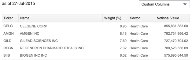
The iShares Nasdaq Biotechnology ETF objective seeks to track the investment results of an index composed of biotechnology and pharmaceutical equities listed on the NASDAQ. It holds 145 different biotech stocks and is market-cap-weighted, so its exposure is more focused on the larger companies. It therefore has two potential disadvantages: it has less exposure to smaller and possibly faster growing biotech stocks and it only holds those stocks listed on the NASDAQ, so it misses some of the companies that may have moved to the NYSE. According to iShares we can see that Biogen (BIIB) is one of the top 5 holdings in the index ETF.

Source: http://www.ishares.com/us/products/239699/ishares-nasdaq-biotechnology-etf

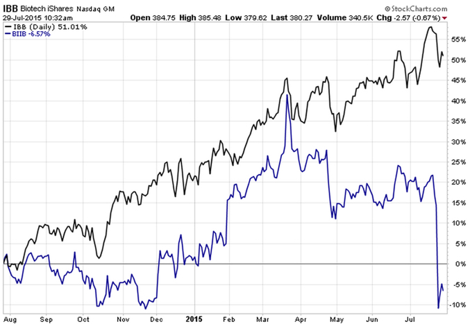
Below is a price chart of the popular iShares Nasdaq Biotech ETF (IBB: the black line) compared to the individual stock Biogen (BIIB: the blue line). Clearly, the more diversified biotech index has demonstrated a more profitable and smoother trend over the past year. And, notice it didn’t experience the recent -30% drop that wiped out Biogen’s price gain. Though some portfolio managers may perceive we can earn more return with individual stocks, clearly that isn’t always the case. Sometimes getting more granular in exposures can instead lead to worse and more volatile outcomes.

Source: Shell Capital Management, LLC created with http://www.stockcharts.com

The nice thing about index ETFs is we have a wide range of them from which to research and choose to add to our investable universe. For example, when I observe the directional price trend in biotech is strong, I can then look at all of the other biotech index ETFs to determine which would give me the exposure I want to participate in the trend.

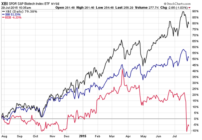
Since we’ve observed with Biogen the magnitude of the potential individual risk of a single biotech stock, that also suggests we may not even prefer to have too much overweight in any one stock within an index. Below I have added to the previous chart the SPDR^® S&P^® Biotech ETF (XBI: the black line) which has about 105 holdings, but the positions are equally-weighted which tilts it toward the smaller companies, not just larger companies. As you can see by the black line below, over the past year, that equal weighting tilt has resulted in even better relative strength. However, it also had a wider range (volatility) at some points. Though it doesn’t always work out this way, you are probably beginning to see how different exposures create unique return streams and risk/reward profiles.

Source: Shell Capital Management, LLC created with http://www.stockcharts.com

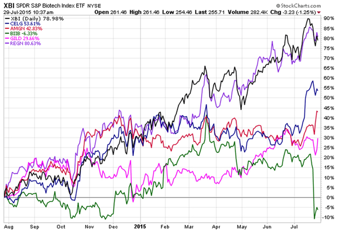
In fact, those who have favored “stock picking” may be fascinated to see the equal-weighted SPDR^® S&P^® Biotech ETF (XBI: the black line) has actually performed as good as the best stock of the top 5 largest biotech stocks in the iShares Nasdaq Biotech ETF.

Source: Shell Capital Management, LLC created with http://www.stockcharts.com

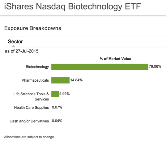
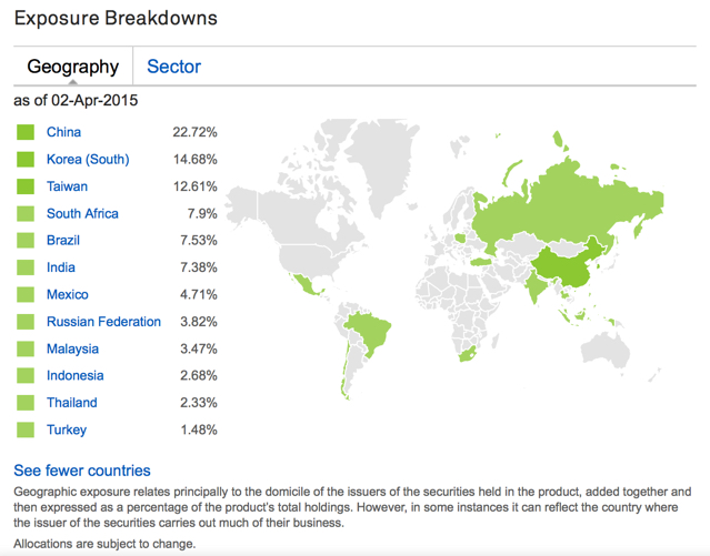
Biotech indexes aren’t just pure biotech industry exposure. They also have exposures to the healthcare sector. For example, iShares Nasdaq Biotech shows about 80% in biotechnology and 20% in sectors categorized in other healthcare industries.

Source: www.ishares.com

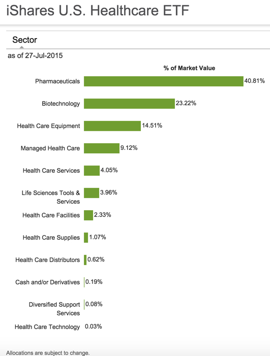
The brings me to another point I want to make. The broader healthcare sector also includes some biotech. For example, the iShares U.S. Healthcare ETF is one of the most traded and includes 23.22% in biotech.

Source: https://www.ishares.com/us/products/239511/IYH?referrer=tickerSearch

It’s always easy to draw charts and look at price trends retroactively in hindsight. If we only knew in advance how trends would play out in the future we could just hold only the very best. In the real world, we can only identify trends based on probability and by definition, that is never a sure thing. Only a very few of us really know what that means and have real experience and a good track record of actually doing it.

I have my own ways I aim to identify potentially profitable directional trends and my methods necessarily needs to have some level of predictive ability or I wouldn’t bother. However, in real world portfolio management, it’s the exit and risk control, not the entry, the ultimately determines the outcome. Since I focus on the exposure to risk at the individual position level and across the portfolio, it doesn’t matter so much to me how I get the exposure. But, by applying my methods to more diversified index ETFs across global markets instead of just U.S. stocks I have fewer individual downside surprises. I believe I take asset management to a new level by dynamically adapting to evolving markets. For example, they say individual selection risk can be diversified away by holding a group of holdings so I can efficiently achieve that through one ETF. However, that still leaves the sector risk of the ETF, so it requires risk management of that ETF position. They say systematic market risk can’t be diversified away, so most investors risk that is left is market risk. I manage both market risk and position risk through my risk control systems and exits. For me, risk tolerance is enforced through my exits and risk control systems.

The performance quoted represents past performance and does not guarantee future results. Investment return and principal value of an investment will fluctuate so that an investor’s shares, when sold or redeemed, may be worth more or less than the original cost. Current performance may be lower or higher than the performance quoted, and numbers may reflect small variances due to rounding. Standardized performance and performance data current to the most recent month end may be obtained by clicking the “Returns” tab above.

Uncharted Territory from the Fed Buying Stocks

August 1, 2015 By Mike Shell in Absolute Return, Absolute Returns, Actively Manage Risk, Adapting to Change, Asymmetric Hedging, Asymmetric Observation, Average Length of Bull Bear Market, Business Cycle, Critical Thinking, Crowd Psychology, Dynamic Hedging, Fed Decision, Investor Behavior Modification, Positive Asymmetry, Risk Asymmetry, The Fed (FOMC) Leave a comment

I remember sometime after 2013 I told someone “The Fed is buying stocks and that’s partly why stocks have risen so surprisingly for so long”. He looked puzzled and didn’t seem to agree, or understand.

The U.S. Federal Reserve (the “Fed”) has been applying “quantitative easing” since the 2007 to 2009 “global financial crisis”. Quantitative easing (QE) is a type of monetary policy used by central banks to stimulate the economy when standard monetary policy has become ineffective. The Fed implements quantitative easing by buying financial assets from banks and other financial institutions. That raises the prices of those financial assets and lowers their interest rate or yield. It also increases the amount of money available in the economy. The magnitude they’ve done this over the past seven years has never been experience before. They are in uncharted territory.

I was reminded of what I said, “the Fed is buying stocks” when I read comments from Bill Gross in “Gross: Fed Slowly Recognizing ZIRP Has Downside Consequences”. He says companies are using easy money to buy their own stock:

Low interest rates have enabled Corporate America to borrow hundreds of billions of dollars “but instead of deploying the funds into the real economy,they have used the proceeds for stock buybacks. Corporate authorizations to buy back their own stock are running at an annual rate of $1.02 trillion so far in 2015, 18 percent above 2007’s record total of $863 billion, Gross said.

You see, if we want to know the truth about market dynamics; we necessarily have to think more deeply about how markets interact. Market dynamics aren’t always simple and obvious. I said, “The Fed is buying stocks” because their actions is driving the behavior of others. By taking actions to increase money supply in the economy and keep extremely low borrowing rates, the Fed has been driving demand for stocks.

But, it isn’t just companies buying their own stock back. It’s also investors buying stocks on margin. Margin is borrowed money that is used to purchase securities. At a brokerage firm it is referred to as “buying on margin”. For example, if we have $1 million in a brokerage account, we could borrow another $1 million “on margin” and invest twice as much. We would pay interest on the “margin loan”, but those rates have been very low for years. Margin interest rates have been 1 – 2%. You can probably see the attraction. If we invested in lower risk bonds earning 5% with $1 million, we would normally earn 5%, or $50,000 annually. If we borrowed another $1 million at 2% interest and invested the full $2 million at 5%, we would earn another 3%, or $30,000. The leverage of margin increased the return to 8%, or $80,000. Of course, when the price falls, the loss is also magnified. When the interest rate goes up, it reduces the profit. But rates have stayed low for so long this has driven margin demand.

While those who have their money sitting in in bank accounts and CDs have been brutally punished by near zero interest rates for many years, aggressive investors have borrowed at those low rates to magnify their return and risk in their investments. The Fed has kept borrowing costs extremely low and that is an incentive for margin.

In the chart below, the blue line is the S&P 500 stock index. The red line is NYSE Margin Debt. You may see the correlation. You may also notice that recessions (the grey area) occur after stock market peaks and high margin debt balances. That’s the downside: margin rates are at new highs, so when stocks do fall those investors will either have to exit their stocks to reduce risk or they’ll be forced to exit due to losses. If they don’t have a predefined exit, their broker has one for them: “a margin call”.

Source: http://www.advisorperspectives.com/dshort/charts/markets/nyse-margin-debt.html?NYSE-margin-debt-SPX-since-1995.gif

If you noticed, I said, “They are in uncharted territory”. I am not. I am always in uncharted territory, so I never am. I believe every new moment is unique, so I believe everyone is always in uncharted territory. Because I believe that, I embrace it. I embrace uncertainty and prepare for anything that can happen. It’s like watching a great movie. It would be no fun if we knew the outcome in advance.

Low Volatility and Managed Volatility Smart Beta is Really Just a Shift in Sector Allocation

July 30, 2015 By Mike Shell in Absolute Return, ETF Strategist, Managed Volatility, Sector ETF, Sector Rotation, Sector Trends, Tactical ETF Managed Portfolio Leave a comment

There is a lot of talk nowadays about “Smart Beta”. Smart beta refers to an investment style where the manager passively follows an index designed to take advantage of perceived systematic biases or inefficiencies in the market. Smart beta defines a set of investment strategies that emphasize the use of alternative index construction rules to traditional market capitalization based indices.

Low volatility or managed volatility, for example, is considered a version of “smart beta” because its weights the stocks (and therefore sector exposure) differently:

The PowerShares S&P 500^® Low Volatility Portfolio (Fund) is based on the S&P 500^®Low Volatility Index (Index). The Fund will invest at least 90% of its total assets in common stocks that comprise the Index. The Index is compiled, maintained and calculated by Standard & Poor’s and consists of the 100 stocks from the S&P 500^® Index with the lowest realized volatility over the past 12 months. Volatility is a statistical measurement of the magnitude of up and down asset price fluctuations over time. The Fund and the Index are rebalanced and reconstituted quarterly in February, May, August and November.

I bolded the main difference between this index ETF and the traditional capitalization-weighted S&P 500. The S&P 500 everyone knows about weights is 500 stocks holdings based on market capitalization, so the largest stocks are the largest positions in the index.

The Low Volatility Portfolio is really a play on sector allocation. Because it creates its position size based on each stocks past 12 months volatility, it’s weighting will simply depend on what was less volatile the past year. And, it will look back to rebalance and reconstitute quarterly in February, May, August and November. So, you may consider what it really does is shifts the position size and sector weighting.

Below is the index sector allocation for the S&P 500 like what is used for SPDR^® S&P 500^® ETF so we can see which sectors have the largest position size.

Source: https://www.spdrs.com/product/fund.seam?ticker=spy

Now we observe the sector allocation of the PowerShares S&P 500 Low Volatility Portfolio. Notice is is heavily weighted in Financials (36%) and Consumer Staples (21%). That’s simply because those sectors stocks have demonstrated less realized volatility as measured by standard deviation over the past 12 months.

Source: https://www.invesco.com/portal/site/us/financial-professional/etfs/product-detail?productId=SPLV

Now, let’s observe the difference in return streams. Below is a relative strength comparison of the two since inception of PowerShares S&P 500^® Low Volatility Portfolio in May 2011. As you see, the low volatility index did have a smaller drawdown in 2011, but overall they’ve tracked the same most of the time. The real difference was the lower drawdown from the sector weighting helped reduce the loss in 2011 and that helped smooth out the returns for a few years. Since 2013 U.S. stock volatility declined, so that explains why the two indexes have trended more closely since.

Source: Shell Capital Management, LLC with http://www.stockcharts.com

Over the past year, there is a little more divergence at times as we see below.

Source: Shell Capital Management, LLC with http://www.stockcharts.com

You may consider that past realized volatility may not repeat into the future. In fact, it could reverse. But the real difference between these is the trailing realized volatility weighting changes the sector weighting. The sectors are the driver. Which sectors have the lowest 12 month historical volatility will determine the exposure to a volatility weighted index or fund. The risk to volatility weighting is the volatility of markets sometimes reach its lowest point at its peak in price as investors become more and more complacent and less indecisive, which is what causes a wider range in prices. I explained this in This is When MPT and VaR Get Asset Allocation and Risk Measurement Wrong.

Though the widening range of prices up and down gets our attention, it isn’t really volatility that investors want to manage so much as it is the downside loss of capital. I really manage volatility by actively increasing and decreasing exposure to loss.

Mike Shell is the Founder and Chief Investment Officer of Shell Capital Management, LLC, and the portfolio manager of ASYMMETRY® Global Tactical.

Mike Shell and Shell Capital Management, LLC is a registered investment advisor and provides investment advice and portfolio management exclusively to clients with a signed and executed investment management agreement. The observations shared on this website are for general information only and are not specific advice, research, or buy or sell recommendations for any individual. For informational purposes only and should not be construed as advice to buy or sell any security. Securities reflected are not intended to represent any client holdings or any recommendations made by the firm. Investing involves risk including the potential loss of principal an investor must be willing to bear. Past performance is no guarantee of future results. All information provided is deemed reliable, but is not guaranteed and should be independently verified. The presence of this website on the Internet shall in no direct or indirect way raise an implication that Shell Capital Management, LLC is offering to sell or soliciting to sell advisory services to residents of any state in which the firm is not registered as an investment advisor. Use of this website is subject to its terms and conditions.

Human judgment, good and bad, will drive investment decisions and financial-market outcomes for the rest of our lives and beyond.

July 23, 2015 By Mike Shell in Absolute Return, Asymmetric Investment Returns, Investor Behavior Modification Tags: Investor Behavior Leave a comment

Source: http://www.project-syndicate.org/commentary/will-computer-algorithms-replace-humans-in-financial-markets-by-robert-j–shiller-2015-07#hmXdmoDjMyvHOw9U.99

Fear is Driving Stock Trend…

July 9, 2015 By Mike Shell in Absolute Return, Absolute Return Investment, Absolute Return Objective, Absolute Returns, Actively Manage Risk, Adapting to Change, Global Directional Trends, Investor Sentiment Leave a comment

Fear is now driving the stock market. As prices fall, investor sentiment indicators suggest that fear increases as prices fall. When sentiment gets to an extreme it often reverses, or it can become contagion and drive prices even lower as people sell their positions. Now that most sentiment gauges are at short term “Extreme Fear” readings, don’t be surprised to see prices trend back up. If they don’t, then it could be the early stages of a larger decline as fear and greed can always get even more extreme.

A simple gauge for investor sentiment is the CNN Money Fear & Greed Index.

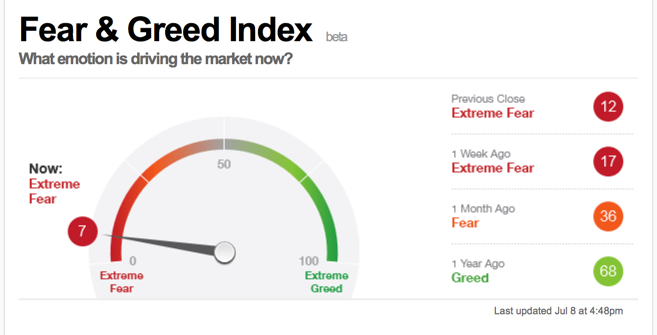
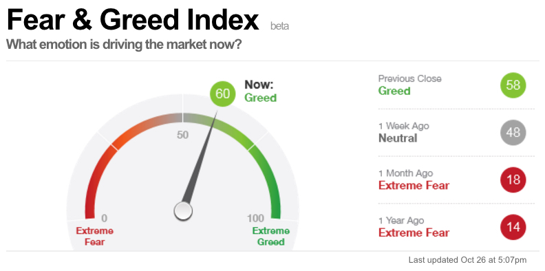Source: http://money.cnn.com/data/fear-and-greed/

It’s always a good time to manage, direct, and control risk. I do that by predefining my exits and knowing how much potential loss that represents in each position and across the portfolio.

Global Stock Market Trends

June 29, 2015 By Mike Shell in Absolute Return, Actively Manage Risk, Adapting to Change, Asymmetric Observation, Global Directional Trends Leave a comment

Stock markets around the world declined -2% or so arguing over which flag to fly. It was a good day for a cash position, or something other than U.S. and International stocks. Below is a table of U.S. stock sectors.

Source: http://www.sectorspdr.com/sectorspdr/tools/sector-tracker

But it wasn’t just U.S. stocks. Equity markets around the globe were down. The graphic below shows much of the world stock markets down around -4%. Spain and Germany were down the most.

Source: http://www.etf.com

The big news came over the weekend that Greece closed banks to head off chaos as bailout talks break down. Greece owes lenders $242.8 billion Euros in total and $1.7 billion tomorrow. Germany is its largest creditor.

The Greek stock market is closed, but the ETFs are not. The Global X FTSE Greece 20 ETF (GREK) was down nearly -20%. The Global X FTSE Greece 20 ETF tracks the FTSE/ATHEX Custom Capped Index, which is designed to reflect broad based equity market performance in Greece. The index is comprised of the top 20 companies listed on the Athens Exchange by market capitalization.

Much of the world is in great debt…

One day isn’t much of a trend, but -2% days like this are notable, so we’ll see if it is the beginning of a trend. The year-to-date total return (including dividends) is negative for both the Dow Jones Industrial Average and the IBoxx $ Invest Grade Corporate Bond ETF.

The stock market is risky and that includes the loss of capital. Past performance does not guarantee future results.

Why Dividend Stocks are Not Always a Safe Haven

June 8, 2015 By Mike Shell in Absolute Return, Actively Manage Risk, Adapting to Change, Asymmetric Investment Returns, Global Directional Trends, Independent Thinking, Sector Rotation, Sector Trends, Systematic Global Macro, Tactical Asset Allocation, Tactical ETF Managed Portfolio, Trend Following 2 Comments

We often hear that high dividend stocks are a “safe haven” in market downtrends. The theory is the yield paid from dividend stocks offset losses in their price. Another theory is that money rotates out of risky assets into those perceived to be less risky: stocks that pay high dividends tend to be older cash rich companies that pay out their cash as dividends. In theory, that sounds “safer”.

I like to point out logical inconsistencies: when beliefs contradict reality.

The above may be true in some cases and it sounds like a good story. In reality, everything changes. The universe is transient, in a constant state of flux. This impermanence, that things are constantly changing and evolving, is one of the few things we can be sure about. It’s a mistake to base too much of an investment strategy on something that has to continue to stay the same. It’s an edge to be adaptive in response to directional trends.

Below is the year-to-date chart iShares Select Dividend ETF that seeks to track the investment results of an index composed of relatively high dividend paying U.S. equities. Notice that I included both the price change by itself (blue) and the total return that includes price plus dividends (orange). The “help” from the dividend over the past six months has helped a little. The price is down -3% but factoring in the dividend leaves the index down -2.33% for the year. The 0.7% is the dividend yield so far.

What has probably gotten investors attention, however, isn’t that their dividend stocks are down over -2% for the year, but that they are down over -4% off their high. That doesn’t sound like a lot: unless you are a conservative investor expecting a “safe haven” from high dividend yielding stocks…

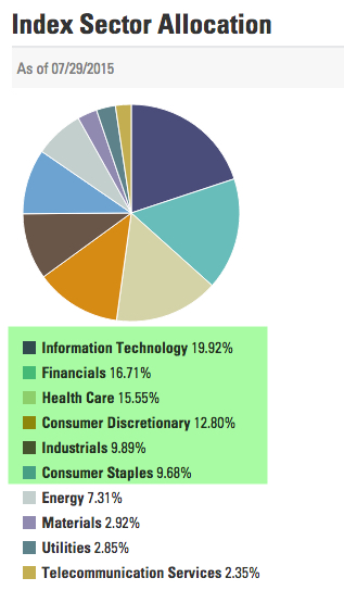
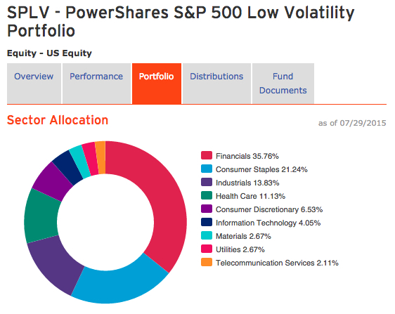
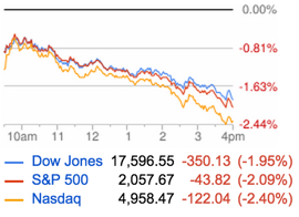
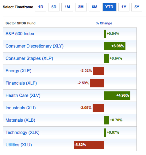
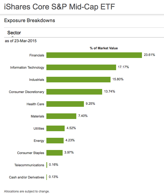
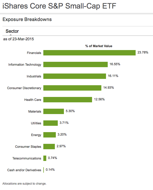
In contrast, the Dow Jones Industrial Average is up about 1% over the same period – counting dividends. You may be wondering what is causing this divergence? Below is the sector holdings for the iShares Select Dividend ETF.

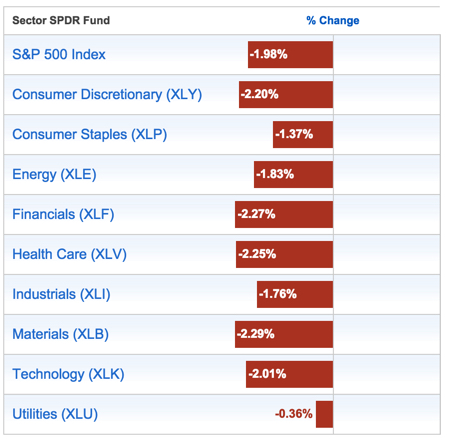
The position size matters and makes all the difference. Notice in the table above the Utilities, Consumer Staples, and Energy Sectors are the top holdings of the index. As you see below, the Utilities sector is down nearly -9% year-to-date, Energy and Staples are down over -1%. They are the three worst performing sectors…

Source: Created by ASYMMETRY® Observations with www.stockcharts.com

Wondering what may be driving it? For the Utility sector it’s probably interest rates. You can read about that in What You Need to Know About Long Term Bond Trends. I prefer to rotate between sectors based on their directional price trends rather than just allocate to them with false hope they may do something they may not.

What You Need to Know About Long Term Bond Trends

June 6, 2015 By Mike Shell in Absolute Return, Absolute Returns, Actively Manage Risk, Adapting to Change, Alternative Investment, Asymmetric Risk Reward, Average Length of Bull Bear Market, Business Cycle, Counter trend, Empirical Observation, ETF Strategist, Global Asset Allocation, Global Directional Trends, Global Macro, Global Tactical Rotation, Hiring a Portfolio Manager, Mean Reversion, Momentum Relative Strength, Quantitative Evidence-Based Rearch, Risk Asymmetry, Sector Trends, Tactical ETF Managed Portfolio, The Fed (FOMC) Leave a comment

There is a lot of talk about interest rates and bonds these days – for good reason. You see, interest rates have been in a downtrend for decades (as you’ll see later). When interest rates are falling, the price of bonds go up. I wrote in “Why So Stock Market Focused?” that you would have actually been better off investing in bonds the past 15 years over the S&P 500 stock index.

However, the risk for bond investors who have a fixed bond allocation is that interest rates eventually trend up for a long time and their bonds fall.

This year we see the impact of rising rates and the impact of falling bond prices in the chart below of the 20+ year Treasury bond. It’s down -15% off its high and since the yield is only around 2.5% the interest only adds about 1% over this period for a total return of -14.1%. Up until now, this long term Treasury index has been a good crutch for a global allocation portfolio. Now it’s more like a broken leg.

But, that’s not my main point today. Let’s look at the bigger picture. Below is the yield (interest rate) on the 10-Year U.S. government bond. Notice that the interest rate was as high as 9.5% in 1990 and has declined to as low as 1.5%. Just recently, it’s risen to 2.62%. If you were going to buy a bond for future interest income payments, would you rather invest in one at 9.5% or 1.5%? If you were going to lend money to someone, which rate would you prefer to receive? What is a “good deal” for you, the lender?

I like trends and being positioned in their direction since trends are more likely to continue than reverse, but they usually do eventually reverse when inertia comes along (like the Fed). If you care about managing downside risk you have to wonder: How much could this trend reverse and what could its impact be on fixed bond holdings? Well, we see below that the yield has declined about -70%. If we want to manage risk, we have to at least expect it could swing the other way.

One more observation. Germany is one of the largest countries in the world. Since April, the 10-year German bond interest rate has reversed up very sharp. What if U.S bonds did the same?

As I detailed in “Allocation to Stocks and Bonds is Unlikely to Give us What We Want” bonds are often considered a crutch for a global asset allocation portfolio. If you care about managing risk, you may consider that negative correlations don’t last forever. All trends change, eventually. You may also consider your risk of any fixed positions you have. I prefer to actively manage risk and shift between global markets based on their directional trends rather than a fixed allocation to them.

The good news is: by my measures, many bond markets have declined in the short term to a point they should at least reserve back up at least temporarily. What happens after that will determine if the longer trend continues or begins to reverse. The point is to avoid complacency and know in advance at what point you’ll exit to cut losses short…

As they say: “Past performance is no guarantee of the future“.

A Random Walker on Stock and Bond Valuation

June 2, 2015 By Mike Shell in Absolute Return, Absolute Return Strategy, Absolute vs. Relatative Return, Actively Manage Risk, Adapting to Change, Asymmetric Investment Returns, Global Directional Trends, Global Macro, Global Tactical Rotation, Liquid Alternative, Sector ETF, Tactical Asset Allocation, Tactical ETF Managed Portfolio Tags: Bond Market Valuation, Stock Market Valuation Leave a comment

Burton Malkiel is a passive buy and hold investor who believes markets are random. To believe markets are random is to believe there are no directional trends, or high or low valuations. He is the author of “A Random Walk Down Wall Street“. But in today’s Wall Street Journal even the ” Random Walker” sees that stock valuations are high and future expected returns low, but believes if there is a bubble it’s in bonds.

BURTON G. MALKIEL

June 1, 2015 6:58 p.m. ET

“Stock valuations are well above their average valuation metrics of the past, and future returns are likely to be below historical averages. But even as Ms. Yellen talks of gradually ending the Fed’s near-zero interest rate policy, interest rates remain well below historical norms. If there is a market bubble today, it is in the bond market and the Fed is complicit in the “overvaluation.”

Source: http://www.wsj.com/articles/janet-yellen-is-no-stock-market-sage-1433199503

When someone invests in bonds for the long term they mainly intend to earn interest. So, bond investors want to buy bonds when yields are high. In the chart below, I show the iShares iBoxx $ Investment Grade Corporate Bond index ETF that seeks to track the investment results of an index composed of U.S. dollar-denominated, investment grade corporate bonds. The blue line is its price trend, the orange line is the index yield. We observe the highest yield was around 5.33% during a spike in 2008 when the price declined. Fixed income has interest-rate risk. Typically, when interest rates rise, there is a corresponding decline in bond values. Since 2008, interest rates and the yield of this bond index has declined. Clearly, the rate of “fixed income” from bonds depends on when you buy them. Today, the yield is only 2.8%, so for “long term allocations” bonds aren’t nearly as attractive as they where.

Another observation is the iShares 20+ Year Treasury Bond ETF, which seeks to track the investment results of an index composed of U.S. Treasury bonds with remaining maturities greater than twenty years. So, this index is long term government bonds. Below we see its yield was 4.75% a decade ago and is now only 2.27%. Buying it to get a 4.75% yield is a very different expected return than 2.27%.

However, that doesn’t mean we can’t tactically rotate between these bond markets trying to capture price trends rather than allocate to them.

Chart source: http://www.ycharts.com

Seasonal Alpha? The Real Probability and Expectation of “Sell in May and Go Away”

May 30, 2015 By Mike Shell in Absolute Return, Absolute Return Fund, Absolute Return Investing, Absolute Return Investment, Absolute Return Objective, Absolute Return Strategy, Absolute Returns, Asymmetric Observation, Global Directional Trends Tags: Seasonal Alpha, Seasonal Strategy 2 Comments

Here is the trouble with a seasonal strategy. According to Standard & Poors, the S&P 500 has gained 1.05 % in May, though it was a volatile month. So, “sell in May and go away” just missed out for no other reason other than it was May.

The second problem is best explained in the chart below. According to Standard & Poors, since 1946 (68 years) the S&P 500 has actually been positive during the “sell in May and go away” period May – October 64% of the time with an average gain of 1.3%. So, the expectation for the period is actually a positive return of .83% May to October.

Another interesting observation in the chart is after a positive “up” May, the May to October period tends to increase 87% of the time an average of 3.5%. So, the expectation is 3.04%. Based on the probability and expectation, we would expect 2% more through October. Of course, the trouble is this stock index is trading at 27 times EPS which is overvalued territory, so this time could instead be the 13% of the time it declines instead, but the probability and expectation is what it is and we want to invest with it, not against it. I would rather focus on the actual direction of trends rather than what month it is.

One month or series of months is an arbitrary time frame, which is why a strategy based on specific time frames like “Sell in May and Go Away” are arbitrary – no matter what story is told to make it sound good.

This May it turned out it most of the other global markets were down materially in May like the Emerging Markets index -4.1%, Commodity Index -2.17%, and even the iShares iBoxx $ Investment Grade Corporate Bond declined -1.12%. So, anyone who was globally positioned across multiple markets during May did experience declines. Those who shifted from the S&P 500 index to bonds at the beginning of May actually lost what the stock index gained…

I prefer to focus on the actual direction of global price trends, no matter when they are. You can see what that looks like here.

Allocation to Stocks and Bonds is Unlikely to Give us What We Want

May 23, 2015 By Mike Shell in Absolute Return, Absolute Return Fund, Absolute Return Investing, Absolute Return Investment, Absolute Return Objective, Absolute Return Strategy, Absolute Returns, Absolute vs. Relatative Return, Actively Manage Risk, Adapting to Change, Alternative Investment, Asymmetric Investment Returns, Asymmetric Observation, Asymmetric Risk Reward, Average Length of Bull Bear Market, Global Asset Allocation, Tactical ETF Managed Portfolio Leave a comment

That was the lesson you learned the last time stocks became overvalued and the stock market entered into a bear market.

I believe holding and re-balancing markets doesn’t give us the risk-adjusted returns we want. In all I do, I believe in challenging that status quo, I believe in thinking and doing things differently. The way I challenge the status quo is a focus on absolute return, limiting downside risk, and doing it tactically across global markets. Why do I do it?

In a Kiplinger article by Fred W. Frailey interviewed Mohamed El-Erian, the PIMCO’s boss, (PIMCO is one of the largest mutual fund companies in the world) he says “he tells how to reduce risk and reap rewards in a fast-changing world.” This article “Shaking up the Investment Mix” was written in March 2009, which turned out the be “the low” of the global market collapse.

It is useful to revisit such writing and thoughts, especially since the U.S. stock market has since been overall rising for 5 years and 10 months. It’s one of the longest uptrends recorded and the S&P 500 stock index is well in “overvalued” territory at 27 times EPS. At the same time, bonds have also been rising in value, which could change quickly when rates eventually rise. At this stage of a trend, asset allocation investors could need a reminder. I can’t think of a better one that this:

Why are you telling investors they need to diversify differently these days?

The traditional approach to diversification, which served us very well, went like this: Adopt a diversified portfolio, be disciplined about rebalancing the asset mix, own very well-defined types of asset classes and favor the home team because the minute you invest outside the U.S., you take on additional risk. A typical mix would then be 60% stocks and 40% bonds, and most of the stocks would be part of Standard & Poor’s 500-stock index.

This approach is fatigued for several reasons. First of all, diversification alone is no longer sufficient to temper risk. In the past year, we saw virtually every asset class hammered. You need something more to manage risk well.

But, you know, they say a picture is worth a thousand words.

Since we are talking about downside risk, something that is commonly hidden when only “average returns” are presented, below is a drawdown chart. I created the drawdown chart using YCharts which uses total return data and the “% off high”. The decline you see from late 2007 to 2010 is a drawdown: it’s when the investment value is under water. Think of this like a lake. You can see how the average of the data wouldn’t properly inform you of what happens in between.

First, I show PIMCO’s own allocation fund: PALCX: Allianz Global Allocation Fund. I include an actively managed asset allocation that is very large and popular with $55 billion invested in it: MCLOX: BlackRock Global Allocation. Since there are many who instead believe in passive indexing and allocation, I have also included DGSIX: DFA Global Allocation 60/40 and VBINX: Vanguard Balanced Fund. As you can see, they have all done about the same thing. They declined about -30% to -40% from October 2007 to March 2009. They also declined up to -15% in 2011.

Going forward, the next bear market may be very different. Historically, investors consider bond holdings to be a buffer or an anchor to a portfolio. When stock prices fall, bonds haven’t been falling nearly as much. To be sure, I show below a “drawdown chart” for the famous actively managed bond fund PIMCO Total Return and for the passive crowd I have included the Vanguard Total Bond Market fund. Keep in mind, about 40% of the allocation of the funds above are invested in bonds. As you see, bonds dropped about -5% to -7% in the past 10 years.

You may notice they are recently down -2% from their highs. Based on the past 10 years, that’s just a minor decline. The trouble going forward is that interest rates have been in an overall downtrend for 30 years, so bond values have been rising. If you rely on bonds being a crutch, as on diversification alone, I agree with Mohamed El-Erian the Chief of the worlds largest bond manager:

“…diversification alone is no longer sufficient to temper risk. In the past year, we saw virtually every asset class hammered. You need something more to manage risk well.”

But, don’t wait until AFTER markets have fallen to believe it.

I just don’t believe holding and re-balancing markets is going to give us the risk-adjusted returns we want. In all I do, I believe in challenging that status quo, I believe in thinking and doing things differently. The way I challenge the status quo is a focus on absolute return, limiting downside risk, and doing it tactically across global markets. Want to join us? To see what that looks like, click: ASYMMETRY® Managed Accounts

On Actively Managing Risk… and Persistence

May 9, 2015 By Mike Shell in Absolute Return, Absolute Return Fund, Absolute Return Investing, Absolute Return Investment, Absolute Return Objective, Absolute Return Strategy, Absolute Returns, Absolute vs. Relatative Return, Actively Manage Risk, Adapting to Change, Alternative Investment Strategy, Alternative Trading Strategy, Asymmetric Risk Reward, Global Directional Trends Leave a comment

Source: https://image-store.slidesharecdn.com/c3d3d5ae-e2eb-4e80-9d4c-88e2344b5572-original.jpeg

I just keep doing what I do…

Where is the Inflation?

May 6, 2015 By Mike Shell in Absolute Return, Absolute Return Fund, Absolute Return Investing, Absolute Return Investment, Absolute Return Objective, Absolute Return Strategy, Absolute Returns, Actively Manage Risk, Adapting to Change, Asymmetric Investment Returns, Asymmetric Observation, Global Directional Trends, Independent Thinking Tags: Inflation Leave a comment

In How does monetary policy influence inflation and employment? and bond prices… I pointed out that even the Fed expected their monetary policy to eventually lead to inflation. The problem with economics and economist is they expect a cause and effect, and often their expectations don’t come true. Remember all those newsletters advising to buy gold the last several years? Gold trended up a while, then down. Applying a good trend system to gold may have made money from it, but buying and holding gold is probably a loser. Inflation was supposed to go up and gold was supposed to be a shelter. However, inflation has instead trended down: The U.S. Inflation Calculator presents it best:

Current US Inflation Rates: 2005-2015

The latest inflation rate for the United States is -0.1% through the 12 months ended March 2015 as published by the US government on April 17, 2015. The next update is scheduled for release on May 22, 2015 at 8:30 a.m. ET. It will offer the rate of inflation over the 12 months ended April 2015.

The chart, graph and table below displays annual US inflation rates for calendar years 2004-2014. Rates of inflation are calculated using the current Consumer Price Index published monthly by the Bureau of Labor Statistics (BLS). For 2015, the most recent monthly data (12-month based) will be used in the chart and graph.

Historical inflation rates are available from 1914-2015. If you would like to calculate accumulated rates between different dates, the US Inflation Calculator will do that quickly.

Source: http://www.usinflationcalculator.com/inflation/current-inflation-rates/

However, as you can see in the chart, like market prices, economic data trends directionally too. This trend of declining inflation may continue or it may reverse.

How does monetary policy influence inflation and employment? and bond prices…

Straight from the Federal Reserve website titled How does monetary policy influence inflation and employment?

In the short run, monetary policy influences inflation and the economy-wide demand for goods and services–and, therefore, the demand for the employees who produce those goods and services–primarily through its influence on the financial conditions facing households and firms. During normal times, the Federal Reserve has primarily influenced overall financial conditions by adjusting the federal funds rate–the rate that banks charge each other for short-term loans. Movements in the federal funds rate are passed on to other short-term interest rates that influence borrowing costs for firms and households. Movements in short-term interest rates also influence long-term interest rates–such as corporate bond rates and residential mortgage rates–because those rates reflect, among other factors, the current and expected future values of short-term rates. In addition, shifts in long-term interest rates affect other asset prices, most notably equity prices and the foreign exchange value of the dollar. For example, all else being equal, lower interest rates tend to raise equity prices as investors discount the future cash flows associated with equity investments at a lower rate.

In turn, these changes in financial conditions affect economic activity. For example, when short- and long-term interest rates go down, it becomes cheaper to borrow, so households are more willing to buy goods and services and firms are in a better position to purchase items to expand their businesses, such as property and equipment. Firms respond to these increases in total (household and business) spending by hiring more workers and boosting production. As a result of these factors, household wealth increases, which spurs even more spending. These linkages from monetary policy to production and employment don’t show up immediately and are influenced by a range of factors, which makes it difficult to gauge precisely the effect of monetary policy on the economy.

Monetary policy also has an important influence on inflation. When the federal funds rate is reduced, the resulting stronger demand for goods and services tends to push wages and other costs higher, reflecting the greater demand for workers and materials that are necessary for production. In addition, policy actions can influence expectations about how the economy will perform in the future, including expectations for prices and wages, and those expectations can themselves directly influence current inflation.

In 2008, with short-term interest rates essentially at zero and thus unable to fall much further, the Federal Reserve undertook nontraditional monetary policy measures to provide additional support to the economy. Between late 2008 and October 2014, the Federal Reserve purchased longer-term mortgage-backed securities and notes issued by certain government-sponsored enterprises, as well as longer-term Treasury bonds and notes. The primary purpose of these purchases was to help to lower the level of longer-term interest rates, thereby improving financial conditions. Thus, this nontraditional monetary policy measure operated through the same broad channels as traditional policy, despite the differences in implementation of the policy.

Up until now, the Long Term Treasury bond has typically gained in price on days the U.S. stock market is down. The recent price action may be a sign of changing inter-market dynamics between the Long Term Treasury and U.S. Stocks now that the Fed isn’t buying these bonds as they have for several years. As you can see in the chart below, the iShares Barclays 20+ Year Treasury Bond Index was down -1.7% today as stocks were also down. It’s also in a shorter term downtrend since January. This could be a sign that may not offer the “crutch” for falling stocks they have in the past. In the next bear market, bonds may go down too.

Created with http://www.stockcharts.com

Recent Observations: Stock Market, Volatility, Absolute Returns

May 2, 2015 By Mike Shell in Absolute Return, Absolute Return Objective, Absolute Return Strategy, Actively Manage Risk, Asymmetric Investment Returns, Asymmetric Observation, Global Directional Trends Leave a comment

In case you missed them, here is a list of popular observations I’ve shared recently:

This is When MPT and VaR Get Asset Allocation and Risk Measurement Wrong

A Tale of Two Conditions for U.S. and International Stocks: Before and After 2008

Absolute Return: an investment objective and strategy

Asymmetric Nature of Losses and Loss Aversion

Why So Stock Market Focused?

What About the Stock Market Has Changed? A Look at Ten Years of Volatility

Diversification Alone is No Longer Sufficient to Temper Risk…

Top Traders Unplugged Interview with Mike Shell: Episode 1 & 2

Asymmetric Sector Exposure in Stock Indexes

My 2 Cents on the Dollar, Continued…

May 1, 2015 By Mike Shell in Absolute Return, Absolute Return Investing, Absolute Return Investment, Absolute Return Objective, Absolute Return Strategy, Absolute Returns, Actively Manage Risk, Adapting to Change, Asymmetric Investment Returns, Critical Thinking, Global Directional Trends, Independent Thinking Leave a comment

In My 2 Cents on the Dollar I explained how the U.S. Dollar is a significant driver of returns of other markets. For example, when the U.S. Dollar is rising, commodities like gold, oil, and foreign currencies like the Euro are usually falling. A rising U.S. Dollar also impacts international stocks priced in U.S. Dollars. When the U.S. Dollar trends up, many international markets priced in U.S. Dollars may trend down (reflecting the exchange rate). Many trend followers and global macro traders are likely “long the U.S. Dollar” by being long and short other markets like commodities, international stocks, or currencies.

Below was the chart from My 2 Cents on the Dollar last week to show the impressive uptrend and since March a non-trending indecisive period. After such a period, I suggested the next break often determines the next directional trend.

Chart created by Shell Capital with: http://www.stockcharts.com

Keep in mind, this is looking closely at a short time frame within a larger trend. Below is the updated chart today, a week later. The U.S. Dollar did break down so far, but by my math, it’s now getting to an even more important point that will distinguish between a continuation of the uptrend or a reversal. This is the point where it should reverse back up, if it’s going to continue the prior uptrend.

Chart created by Shell Capital with: http://www.stockcharts.com

This is a good example of understanding what drives reward/risk. I consider how long the U.S. Dollar I am (by being synthetically long/short other markets) and how that may impact my positions if the trend were to reverse. It’s a good time to pay attention to it to see if it breaks back out to the upside to resume the uptrend, or if it instead breaks down to end it.

That’s my two cents on the Dollar… How long are you?

Why So Stock Market Focused?

April 25, 2015 By Mike Shell in Absolute Return, Absolute Return Fund, Absolute Return Investing, Absolute Return Investment, Absolute Return Objective, Absolute Return Strategy, Absolute Returns, Adapting to Change, Alternative Investment Strategy, Alternative Trading Strategy, Asymmetric Investment Returns, Asymmetric Observation, Asymmetric Risk, Asymmetric Risk Reward, Global Directional Trends, Global Macro, Hiring a Portfolio Manager, Independent Thinking, Investor Behavior Modification, Investor Sentiment, Liquid Alternative, Managed Volatility, Sector Rotation, Sector Trends, Secular Bear Market, Secular Bull Market, Systematic Global Macro, Tactical Asset Allocation, Tactical ETF Portfolio Management Leave a comment

Most investors and their advisors seem to speak mostly about the stock market. When they mention “the market” and I ask “what market?” they always reply “the stock market”.

Why so stock market centric?

It must be that it gets the most media attention or stocks seem more exciting?. After all, other markets like bonds may seem boring and few know much about the many commodities markets or the foreign exchange markets. There are many different markets and two sides to them all.

If it’s risk-adjusted returns you want, you may be surprised to find where you should have invested your money the past 15 years. To make the point, below is a comparison of the total return of the Vanguard S&P 500 stock index (the orange line) compared to the Vanguard Bond Index (the blue line). Yes, you are seeing that correctly. Using these simple index funds as a proxy, bonds have achieved the same total return as stocks, but with significantly less volatility and drawdowns. This is why we never look at just “average” return data without considering the path it took to get there. A total return percentage gain chart like this one presents a far more telling story. Take a close look at the path they took.

Created with http://www.ycharts.com

I showed the chart to one investment advisor who commented “It looks like the stock market is catching up”. If that’s what you think of when you view the chart, you may have a bias blind spot: ignoring the vast difference in the risk between the two markets.

Looking at the total return over the period identifies the obvious difference in the path the two return streams took to achieve their results, but below we see the true risk difference. Drawdowns are declines from a higher value to a low value and a visual representation of how long it took to recover the lose of capital. When we observe a drawdown chart like the one below, it’s like a lake. These charts together also help illustrate the flaw of averages. The average return of the stock and bond index have ended at about the same level and have the same average return, but the bond index achieved it with much less drawdown. You wouldn’t know that if you only looked at average returns. If you tried to walk across the stock market lake, you may have drowned if you couldn’t handle swimming in 40′ of water for so long. If that one didn’t get you, the 55′ may have. The stock index declined about -40% from 2000 – 2002 and took years to recover before it declined -55%.

Created with http://www.ycharts.com

You have to be wondering: why didn’t you just invest in bonds 15 years ago? Maybe you were focused on the prior period huge average returns in stocks?

Before I continue, let me place a very bold disclaimer here: PAST PERFORMANCE DOES NOT GUARANTEE FUTURE RESULTS. Another way that is stated is that PAST PERFORMANCE IS NO ASSURANCE OF FUTURE RESULTS. One more version is PAST PERFORMANCE MAY NOT BE AN INDICATION OF FUTURE RESULTS. If you remember, the 1990’s were a roaring bull market in stocks. People focus on the past expecting it to continue. That’s probably why you never thought to invest in bonds instead of stocks.

Some of the largest and most successful hedge funds in the world have done that very thing over this period and longer. But, they didn’t just invest in bonds. They leveraged bonds. We’ve seen in this example that a bond index fund has achieved just as much total return as stocks. If you are a stock market centric investor: one that likes the stock market and makes it your focus, then you necessarily had to be willing to endure those -40% to -55% declines and wait many years to recover from the losses. If you are really willing to accept such risk, imagine if you had used margin to leverage bonds. The bond index rarely declined -10% or more. It was generally a falling interest rate period, so bonds gained value. If you were willing to accept -40% to -55% declines in stocks, you could have instead leveraged the bonds 400% or 500%. If you had done that, your return would be 4 or 5 times more with a downside more equal to that of stocks.

Why so stock centric?

Of course, at this stage, the PAST PERFORMANCE IS HIGHLY UNLIKELY TO REPEAT INTO THE FUTURE. Just as the roaring stocks of the 1990’s didn’t repeat. To see why, read Stage and Valuation of the U.S. Stock Market and Bonds: The Final Bubble Frontier?.

From my observations of investors performance and their advisors, most people seem to have poor results the past decade or so, even after this recent bull market. An investment management consultant told me recently that investors and their advisors who are aware of the current stage of stocks and bonds feel there is no place to turn. I believe it’s a very important time to prepare to row, not sail. For me, that means focus on actively managing risk and look for potentially profitable trends across a very global universe of markets; currency, bonds, stocks, commodities, and alternatives like volatility, inverse, etc . That’s my focus in ASYMMETRY® | Managed Accounts.

Stage and Valuation of the U.S. Stock Market

April 24, 2015 By Mike Shell in Absolute Return, Absolute Return Fund, Absolute Return Investing, Absolute Return Investment, Absolute Return Objective, Absolute Return Strategy, Absolute Returns, Actively Manage Risk, Adapting to Change, Alternative Investment, Asymmetric Investment Returns, Asymmetric Observation, Asymmetric Risk, Average Length of Bull Bear Market, Business Cycle, Critical Thinking, Global Directional Trends, Global Macro, Independent Thinking, Investor Sentiment, Secular Bear Market, Secular Bull Market Leave a comment

In The REAL Length of the Average Bull Market last year I pointed out different measures used to determine the average length of a bull market. Based on that, whether you believe the average bull market lasts 39 months, 50 months, or 68 months, it seems the current one is likely very late in its stage at 73 months. It’s one of the longest, ever.

I normally don’t consider valuations levels like P/E ratios, but they do matter when it comes to secular bull and bear markets (10 to 20 year trends). That’s because long-term bull markets begin at low valuation levels (10 or below) and have ended at historically high levels (around 20). Currently, the S&P 500 is trading at 27. That, along with the low dividend yield, suggests the expected return for holding that index going forward is low.

Ed Easterling of Crestmont Research explains it best:

The stock market gyrated since the start of the year, ending the first quarter with a minimal gain of 0.4%. As a result, normalized P/E was virtually unchanged at 27.3—well above the levels justified by low inflation and interest rates. The current status remains near “significantly overvalued.”

In addition, the forecast by Standard and Poor’s for 2015 earnings per share (EPS) recently took a nosedive, declining 17% during one week in the first quarter. Volatility remains unusually low in its cycle. The trend in earnings and volatility should be watched closely and investors should remain cognizant of the risks confronting an increasingly vulnerable market.

Source: The P/E Report: Quarterly Review Of The Price/Earnings Ratio By Ed Easterling April 4, 2015 Update

It’s always a good time to actively manage risk and shift between global markets rather than allocate to them. To see what that looks like, visit: http://www.asymmetrymanagedaccounts.com/global-tactical/

Bonds: The Final Bubble Frontier?

April 24, 2015 By Mike Shell in Absolute Return, Absolute Return Investing, Absolute Return Investment, Absolute Return Objective, Absolute Return Strategy, Absolute Returns, Asymmetric Observation Leave a comment

No where to turn? This time, it isn’t just that the U.S. stock indexes are very aged in one of the longest bull markets in history and trading in bubble territory at 27 times EPS.

In “Bonds: The Final Bubble Frontier?” Deutsche Bank says:

“We do think bonds are starting to exhibit bubble tendencies with very little value for investors trying to create long-term real returns”

Source: Long – Term Asset Return Study: Bonds: The Final Bubble Frontier?

We’ll see…

The Volatility Index (VIX) is Getting Interesting Again

April 24, 2015 By Mike Shell in Absolute Return, Absolute Return Fund, Absolute Return Investing, Absolute Return Investment, Absolute Return Objective, Absolute Return Strategy, Absolute Returns, Absolute vs. Relatative Return, Absolute vs. Relative Return, Actively Manage Risk, Adapting to Change, Alternative Investment Strategy, Alternative Trading Strategy, Asymmetric Observation, Asymmetric Payoff, Asymmetric Risk, Asymmetric Risk Reward, Asymmetric Sector Exposure, Asymmetric Thinking, Counter trend, Critical Thinking, Dynamic Hedging, ETF Strategist, Global Asset Allocation, Global Directional Trends, Global Macro, Global Tactical Rotation, Hedge Funds, Hiring a Portfolio Manager, Independent Thinking, Investor Behavior Modification, Investor Sentiment, Liquid Alternative, Managed Momentum, Managed Volatility, Mean Reversion, Momentum Relative Strength, Risk Asymmetry, Sector Rotation, Systematic Global Macro, Tactical Asset Allocation, Tactical ETF Managed Portfolio, Tactical ETF Portfolio Management, VIX CBOE Volatility Index, Volatility Trading 1 Comment

In the last observation I shared on the CBOE Volatlity index (the VIX) I had been pointing out last year the VIX was at a low level and then later started trending up. At that time, many volatility traders seemed to think it was going to stay low and keep going lower – I disagreed. Since then, the VIX has remained at a higher average than it had been – up until now. You can read that in VIX® gained 140%: Investors were too complacent.

Here it is again, closing at 12.45 yesterday, a relatively low level for expected volatility of the S&P 500 stocks. Investors get complacent after trends drift up, so they don’t price in so much fear in options. Below we observe a monthly view to see the bigger picture. The VIX is getting down to levels near the end of the last bull market (2007). It could go lower, but if you look closely, you’ll get my drift.

Chart created by Shell Capital with: http://www.stockcharts.com

Next, we zoom in to the weekly chart to get a loser look.

Chart created by Shell Capital with: http://www.stockcharts.com

Finally, the daily chart zooms in even more.

Chart created by Shell Capital with: http://www.stockcharts.com

The observation?

Options traders have priced in low implied volatility – they expect volatility to be low over the next month. That is happening as headlines are talking about stock indexes hitting all time highs. I think it’s a sign of complacency. That’s often when things change at some point.

It also means that options premiums are generally a good deal (though that is best determined on an individual security basis). Rather than selling premium, it may be a better time to buy it.

Let’s see what happens from here…

My 2 Cents on the Dollar

April 23, 2015 By Mike Shell in Absolute Return, Absolute Return Fund, Absolute Return Investing, Absolute Return Investment, Absolute Return Objective, Absolute Return Strategy, Absolute Returns, Absolute vs. Relatative Return, Absolute vs. Relative Return, Actively Manage Risk, Adapting to Change, Alternative Investment, Alternative Trading Strategy, Asymmetric Hedging, Asymmetric Investment Returns, Asymmetric Observation, Asymmetric Payoff, Asymmetric Risk, Asymmetric Risk Reward, Asymmetric Sector Exposure, Business Cycle, Counter trend, Critical Thinking, Dynamic Hedging, ETF Strategist, Global Asset Allocation, Global Directional Trends, Global Macro, Global Tactical Rotation, Hiring a Portfolio Manager, Independent Thinking, Liquid Alternative, Managed Momentum, Managed Volatility, Mean Reversion, Momentum Relative Strength, Positive Asymmetry, Risk Asymmetry, Sector ETF, Sector Rotation, Sector Trends, Systematic Global Macro, Tactical Asset Allocation, Tactical ETF Portfolio Management, Trend Following 2 Comments

The U.S. Dollar ($USD) has gained about 20% in less than a year. We observe it first in the weekly below. The U.S. Dollar is a significant driver of returns of other markets. For example, when the U.S. Dollar is rising, commodities like gold, oil, and foreign currencies like the Euro are usually falling. A rising U.S. Dollar also impacts international stocks priced in U.S. Dollar. When the U.S. Dollar trends up, many international markets priced in U.S. Dollars may trend down (reflecting the exchange rate). The U.S. Dollar may be trending up in anticipation of rising interest rates.

Chart created by Shell Capital with: http://www.stockcharts.com

Now, let’s observe a shorter time frame- the daily chart. Here we see an impressive uptrend and since March a non-trending indecisive period. Many trend followers and global macro traders are likely “long the U.S. Dollar” by being long and short other markets like commodities, international stocks, or currencies.

Chart created by Shell Capital with: http://www.stockcharts.com

This is a good example of understanding what drives returns and risk/reward. I consider how long the U.S. Dollar I am and how that may impact my positions if this uptrend were to reverse. It’s a good time to pay attention to it to see if it breaks back out to the upside to resume the uptrend, or if it instead breaks down to end it. Such a continuation or reversal often occurs from a point like the blue areas I highlighted above.

That’s my two cents on the Dollar…

How long are you? Do you know?

Conflicted News

April 17, 2015 By Mike Shell in Absolute Return, Absolute Return Fund, Absolute Return Investing, Absolute Return Investment, Absolute Return Objective, Absolute Return Strategy, Absolute Returns, Actively Manage Risk, Adapting to Change, Asymmetric Thinking, Business Cycle, Counter trend, Crowd Psychology, ETF Strategist, Global Directional Trends, Hiring a Portfolio Manager, Independent Thinking, Information Asymmetry, Investor Behavior Modification, Investor Sentiment, Tactical Asset Allocation, Tactical ETF Managed Portfolio, Trend Following Leave a comment

This is a great example of conflicted news. Which news headline is driving down stock prices today?

Below is a snapshot from Google Finance::

Trying to make decisions based on news seems a very conflicted way, which is why I instead focus on the absolute direction of price trends.

Absolute Return vs. Relative Return

April 14, 2015 By Mike Shell in Absolute Return, Absolute Return Fund, Absolute Return Investing, Absolute Return Investment, Absolute Return Objective, Absolute Return Strategy, Absolute Returns, Absolute vs. Relatative Return, Absolute vs. Relative Return, Playing with Words, Relative Returns Leave a comment

Absolute: viewed or existing independently and not in relation to other things; not relative or comparative.

Relative: considered in relation or in proportion to something else.

Return: to go or come back, as to a former place, position, or state.

Oops… we don’t want to “return” do we?

Rate of Return: The gain or loss on an investment over a specified period.

So, an Absolute Rate of Return: is the the gain or loss viewed or existing independently and not in relation to other things; not relative or comparative.

Many people seem to have a problem with what I call “relativity“. For example, they love their home, until someone builds a larger and nicer one across the street. Or, they love their car, until their friend drives up in one that seems even better.

You can probably see how these simple words and their meaning leads to many issues people deal with.

To see an absolute return program applied in real life, visit: http://www.asymmetrymanagedaccounts.com/global-tactical/

Asymmetric Returns of World Markets YTD

April 10, 2015 By Mike Shell in Absolute Return, Absolute Return Fund, Absolute Return Investing, Absolute Return Investment, Absolute Return Objective, Absolute Return Strategy, Absolute Returns, Absolute vs. Relatative Return, Absolute vs. Relative Return, Actively Manage Risk, Adapting to Change, Asymmetric Investment Returns, Asymmetric Observation, Business Cycle, Data Driven Rearch, Global Asset Allocation, Global Directional Trends, Managed Momentum, Managed Volatility, Market Breadth, Momentum Relative Strength, Positive Asymmetry, Quantitative Evidence-Based Rearch Leave a comment

As of today, global stock, bond, commodity markets are generating asymmetric returns year to date. The graph below illustrates the asymmetry is negative for those who need these markets to go “up”.

source: http://finviz.com

Asymmetric Nature of Losses and Loss Aversion

April 8, 2015 By Mike Shell in Absolute Return, Absolute Return Fund, Absolute Return Investing, Absolute Return Investment, Absolute Return Objective, Absolute Return Strategy, Absolute Returns, Absolute vs. Relative Return, Actively Manage Risk, Adapting to Change, Alternative Investment Strategy, Alternative Trading Strategy, Asymmetric Hedging, Asymmetric Investment Returns, Asymmetric Observation, Asymmetric Payoff, Asymmetric Risk, Asymmetric Risk Reward, Asymmetric Thinking, Critical Thinking, Dynamic Hedging, Empirical Observation, ETF Strategist, Global Directional Trends, Global Macro, Hedge Funds, Hiring a Portfolio Manager, Independent Thinking, Investor Behavior Modification, Investor Sentiment, Liquid Alternative, Managed Volatility, Positive Asymmetry, Quantitative Evidence-Based Rearch, Risk Asymmetry, Symmetry Tags: Loss Aversion, Prospect Theory 3 Comments

Loss Aversion:

“In prospect theory, loss aversion refers to the tendency for people to strongly prefer avoiding losses than acquiring gains. Some studies suggest that losses are as much as twice as psychologically powerful as gains. Loss aversion was first convincingly demonstrated by Amos Tversky and Daniel Kahneman.”

For most people, losing $100 is not the same as not winning $100. From a rational point of view are the two things the same or different?

Most economists say the two are the same. They are symmetrical. But I think that ignores some key issues.

If we have only $10 to eat on today and that’s all we have, if we lose it, we’ll be in trouble: hungry.

But if we have $10 to eat on and flip a coin in a bet and double it to $20, we may just eat a little better. We’ll still eat. The base rate: survival.

They say rationally the two are the same, but that isn’t true. They aren’t the same. The loss makes us worse off than we started and it may be totally rational to feel worse when we go backward than we feel good about getting better off. I don’t like to go backward, I prefer to move forward to stay the same.

Prospect Theory, which found people experience a loss more than 2 X greater than an equal gain, discovered the experience of losses are asymmetric.

Actually, the math agrees.

You see, losing 50% requires a 100% gain to get it back. Losing it all is even worse. Losses are indeed asymmetric and exponential on the downside so it may be completely rational and logical to feel the pain of losses asymmetrically. Experience the feeling of loss aversions seems to be the reason a few of us manage investment risk and generate a smoother return stream rather than blow up.

To see what the actual application of asymmetry to portfolio management looks like, see: Shell Capital Management, LLC.

A Tale of Two Conditions for U.S. and International Stocks: Before and After 2008

April 6, 2015 By Mike Shell in Absolute Return, Absolute Return Fund, Absolute Return Investing, Absolute Return Objective, Absolute Return Strategy, Absolute Returns, Absolute vs. Relatative Return, Adapting to Change, Alternative Investment Strategy, Alternative Trading Strategy, Asymmetric Observation, Asymmetric Risk Reward, Business Cycle, Counter trend, ETF Strategist, Global Asset Allocation, Global Directional Trends, Global Macro, Global Tactical Rotation, Systematic Global Macro Tags: Emerging Market ETF, Emerging Markets, International ETF, International Markets 2 Comments

In recent conversations with investment advisors, I notice their sentiment has shifted from “cautious and concerned” about world equity markets to “why have they underperformed”. Prior to 2013, most investors and investment advisors were concerned about another 2007 to 2009 level bear market. Now, it seems that caution has faded. Today, many of them seem to be focused on the strong trend of U.S. stocks since mid-2013 and comparing everything else to it.

Prior to October 2007, International stocks were in significantly stronger positive directional trends than U.S. Stocks. I’ll compare the S&P 500 stock index (SPY) to Developed International Countries (EFA). We can visually observe a material change between these markets before 2008 and after, but especially after 2013. That one large divergence since 2013 has changed sentiment.

The MSCI EAFE Index is recognized as the pre-eminent benchmark in the United States to measure international equity performance. It comprises the MSCI country indices that represent developed markets outside of North America: Europe, Australasia and the Far East. For a “real life” example of its price trend, I use the iShares MSCI EAFE ETF (EFA). Below are the country holdings, to get an idea of what is considered “developed markets”.

Source: https://www.ishares.com/us/products/239623/EFA

Below are the price trends of the popular S&P 500 U.S. stock index and the MSCI Developed Countries Index over the past 10 years. Many investors may have forgotten how strong international markets were prior to 2008. Starting around 2012, the U.S. stock market continued to trend up stronger than international stocks. It’s a tale of two markets, pre-2008 and post-2008.

No analysis of a trend % change is complete without also examining its drawdowns along the way. A drawdown measures a drop from peak to bottom in the value of a market or portfolio (before a new peak is achieved). The chart below shows these indexes % off their prior highs to understand their historical losses over the period. For example, these indexes declined -55% or more. The International stock index nearly declined -65%. The S&P 500 U.S. stock index didn’t recover from its decline that started in October 2007 until mid-2012, 5 years later. The MSCI Developed Countries index is still in a drawdown! As you can see, EFA is -24% off it’s high reached in 2007. Including these international countries in a global portfolio is important as such exposure has historically provided greater potential for profits than just U.S. stocks, but more recently they have been a drag.

The International stock markets are divided broadly into Developed Markets we just reviewed and Emerging Countries. The iShares MSCI Emerging Markets ETF (EEM) tracks this index. To get an idea of which countries are considered “Emerging Markets’, you can see the actual exposure below.

https://www.ishares.com/us/products/239637/EEM?referrer=tickerSearch

The Emerging Countries index has reached the same % change over the past decade, but they have clearly taken very different paths to get there. Prior to the “global crisis” that started late 2007, many investors may have forgotten that Emerging Markets countries like China and Brazil were in very strong uptrends. I remember this very well; as a global tactical trader I had exposure to these countries which lead to even stronger profits than U.S. markets during that period. Since 2009, however, Emerging Markets recovered sharply but as with U.S. stocks: they have trended up with great volatility. Since Emerging Markets peaked around 2011 they have traded in a range since. However, keep in mind, these are 10-year charts, so those swings up and down are 3 to 6 months. We’ll call that “choppy”. Or, 4 years of a non-trending and volatile state.

Once again, no analysis of a trend % change is complete without also examining its drawdowns along the way. A drawdown measures a drop from peak to bottom in the value of a market or portfolio (before a new peak is achieved). The chart below shows these indexes % off their prior highs to understand their historical losses over the period. For example, these indexes declined -55% or more. The Emerging Market stock index declined -65%. The S&P 500 U.S. stock index didn’t recover from its decline that started in October 2007 until mid-2012, 5 years later. The MSCI Emerging Countries index is still in a drawdown! As you can see, EFA is -26% off it’s high reached in 2007. As I mentioned before, it recovered sharply up to 2011 but has been unable to move higher in 4 years. Including these Emerging Markets countries in a global portfolio is important as such exposure has historically provided greater potential for profits than just U.S. stocks, but more recently they have been a drag.

Wondering why the tale of two markets before and after 2008? The are many reasons and return drivers. One of them can be seen visually in the trend of the U.S. Dollar. Below is a 10-year price chart of the U.S. Dollar index. Before 2008, the U.S. Dollar was falling, so foreign currencies were rising as were foreign stocks priced in Dollars. As with most world markets, even the U.S. Dollar was very volatile from 2008 through 2011. After 2011 it drifted in a tighter range through last year and has since increased sharply.

The funny thing is, I’ve noticed there are a lot of inflows into currency-hedged ETFs recently. Investors seem to do the wrong thing at the wrong time. For example, they’ll want to hedge their currency risk after it already happened, not before… It’s just like with options hedging: Investors want protection after a loss, not before it happens. Or, people will buy that 20 KW generator for their home after they lose power a few days, not before, and may not need it again for 5 years after they’ve stopped servicing it. So, it doesn’t start when they need it again.

You can probably see why I think it’s an advantage to understand how world markets interact with each other and it’s an edge for me.

Mike Shell is the Founder and Chief Investment Officer of Shell Capital Management, LLC, and the portfolio manager of ASYMMETRY® Global Tactical.

The observations shared on this website are for general information only and are not specific advice, research, or buy or sell recommendations for any individual. Investing involves risk including the potential loss of principal an investor must be willing to bear. Past performance is no guarantee of future results. The presence of this website on the Internet shall in no direct or indirect way raise an implication that Shell Capital Management, LLC is offering to sell or soliciting to sell advisory services to residents of any state in which the firm is not registered as an investment advisor. Use of this website is subject to its terms and conditions.

Stock Market Year-to-Date and First Quarter

April 2, 2015 By Mike Shell in Absolute Return, Absolute Return Fund, Absolute Return Investing, Absolute Return Investment, Absolute Return Objective, Absolute Return Strategy, Absolute Returns, Absolute vs. Relatative Return, Absolute vs. Relative Return, Asymmetric Sector Exposure, Sector ETF, Sector Rotation, Sector Trends, Tactical ETF Managed Portfolio, Tactical ETF Portfolio Management Leave a comment

So far, the U.S. stock market isn’t doing so well. And, the gains and losses over the past quarter have been asymmetric. Consumer Discretionary (12.6% of the S&P 500 index) and Healthcare (14.8% of the S&P 500 index) have barely offset the losses in four other sectors.

Below are the YTD gain and losses for the popular S&P 500 index and each sector in the index.

source: http://www.sectorspdr.com/sectorspdr/tools/sector-tracker

But, that’s just one data point compared to another data point. Such a table would be incomplete without considering the path those gains and losses took to get there.

source: http://www.sectorspdr.com/sectorspdr/tools/sector-tracker/charting

To see the results of asymmetric exposure and risk management in action across a global universe of markets, visit: http://www.asymmetrymanagedaccounts.com/

Performance is historical and does not guarantee future results; current performance may be lower or higher. Investment returns/principal value will fluctuate so that an investor’s shares, when redeemed, may be worth more or less than their original cost. Past performance does not guarantee future results.

“It is impossible to produce a superior performance unless…

April 1, 2015 By Mike Shell in Absolute Return, Absolute Return Investment, Absolute Return Objective, Absolute Return Strategy, Absolute Returns, Absolute vs. Relatative Return, Alternative Investment Strategy, Great Quotes, Investor Behavior Modification, Investor Sentiment 1 Comment

source: http://www.templeton.org

A great quote from my fellow Tennessean, Sir John Templeton:

“It is impossible to produce a superior performance unless you do something different from the majority.”

– Sir John Templeton

Absolute Return: an investment objective and strategy

March 28, 2015 By Mike Shell in Absolute Return, Absolute Return Fund, Absolute Return Investing, Absolute Return Investment, Absolute Return Objective, Absolute Return Strategy, Absolute Returns, Absolute vs. Relatative Return, Absolute vs. Relative Return, Actively Manage Risk, Adapting to Change, Alternative Investment, Alternative Trading Strategy, Asymmetric Investment Returns, ETF Strategist, Hedge Funds, Hiring a Portfolio Manager, Liquid Alternative, Managed Momentum, Managed Volatility, Momentum Relative Strength, Position Sizing, Positive Asymmetry, Relative Returns, Sector ETF, Sector Rotation, Systematic Global Macro, Tactical ETF Managed Portfolio, Trend Following 1 Comment

Absolute Return in its basic definition is the return that an asset achieves over a certain period of time. This measure looks at the appreciation or depreciation (expressed as a dollar amount or a percentage). For example, a $50 stock drifts to $100 is a 100% absolute return. If that same stock drifts back from $100 to $50, its absolute return is -50%.

Absolute Return as an investment objective is one that does not try to track or beat an arbitrary benchmark or index, but instead seeks to generate real profits over a complete market cycle regardless of market conditions. That is, an absolute return objective of positive returns on investment over a market cycle of both bull and bear market periods irrespective of the direction of stock, commodity, or bond markets. Since the U.S. stock market has been generally in a uptrend for 6 years now, other than the -20% decline in the middle of 2011, we’ll now have to expand our time frame for a full market cycle to a longer period. That is, a full market cycle includes both a bull and a bear market.

The investor who has an absolute return objective is concerned about his or her own objectives for total return over a period and tolerance for loss and drawdowns. That is a very different objective than the investor who just wants whatever risk and return a benchmark, allocation, or index provides. Absolute returns require skill and active management of risk and exposure to markets.

Absolute return as a strategy: absolute return is sometimes used to define an investment strategy. An absolute return strategy is a plan, method, or series of maneuvers aiming to compound capital positively and to avoid big losses to capital in difficult market conditions. Whereas Relative Return strategies typically measure their success in terms of whether they track or outperform a market benchmark or index, absolute return investment strategies aim to achieve positive returns irrespective of whether the prices of stocks, bonds, or commodities rise or fall over the market cycle.

Absolute Return Investment Manager

Whether you think of absolute return as an objective or a strategy, it is a skill-based rather than market-based. That is, the absolute return manager creates his or her results through tactical decision-making as opposed to taking what the market is giving. One can employ a wide range of approaches toward an absolute return objective, from price-based trend following to fundamental analysis. In the ASYMMETRY® Managed Accounts, I believe price-based methods are more robust and lead to a higher probability of a positive expectation. Through my historical precedence, testing, and experience, I find that any fundamental type method that is based on something other than price has the capability to stray far enough from price to put the odds against absolute returns. That is, a manager buying what he or she believes is undervalued and selling short what he believes is overvalued can go very wrong if the position is on the wrong side of the trend. But price cannot deviate from itself. Price is the judge and the jury.

To create absolute returns, I necessarily focus on absolute price direction. Not relative strength, which is a rate of change relative to another moving trend. And, I focus on actual risk, not some average risk or an equation that oversimplifies risk like standard deviation.

Of course, absolute return and the “All Weather” type portfolio sound great and seem to be what most investors want, but it requires incredible skill to execute. Most investors and advisors seem to underestimate the required skills and experience and most absolute return strategies and funds have very limited and unproven track records. There is no guarantee that these strategies and processes will produce the intended results and no guarantee that an absolute return strategy will achieve its investment objective.

For an example of the application of an absolute return objective, strategy, and return-risk profile, visit http://www.asymmetrymanagedaccounts.com/

Absolute Return as an Investment Strategy

March 27, 2015 By Mike Shell in Absolute Return, Absolute Return Fund, Absolute Return Investing, Absolute Return Investment, Absolute Return Objective, Absolute Return Strategy, Absolute Returns, Absolute vs. Relatative Return, Absolute vs. Relative Return, Alternative Investment Strategy, Alternative Trading Strategy, Asymmetric Investment Returns, ETF Strategist, Global Asset Allocation, Global Directional Trends, Global Macro, Hedge Funds, Hiring a Portfolio Manager, Liquid Alternative, Managed Momentum, Managed Volatility, Momentum Relative Strength, Relative Returns, Sector ETF, Sector Rotation, Sector Trends, Tactical ETF Portfolio Management, Trend Following Leave a comment

In “Absolute Return: The Basic Definition”, I explained an absolute return is the return that an asset achieves over a certain period of time. To me, absolute return is also an investment objective.

In “Absolute Return as an Investment Objective” I explained that absolute return is an investment objective is one that does not try to track or beat an arbitrary benchmark or index, but instead seeks to generate real profits over a complete market cycle regardless of market conditions. That is, it is focused on the actual total return the investor wants to achieve and how much risk the investor will willing to take, rather than a focus on what arbitrary market indexes do.

Absolute return as a strategy: absolute return is sometimes used to define an investment strategy. An absolute return strategy is a plan, method, or series of maneuvers aiming to compound capital positively and to avoid big losses to capital in difficult market conditions. Whereas Relative Return strategies typically measure their success in terms of whether they track or outperform a market benchmark or index, absolute return investment strategies aim to achieve positive returns irrespective of whether the prices of stocks, bonds, or commodities rise or fall over the market cycle.

Whether you think of absolute return as an objective or a strategy, it is a skill-based rather than market-based. That is, the absolute return manager creates his or her results through tactical decision-making as opposed to taking what the market is giving. One can employ a wide range of approaches toward an absolute return objective, from price-based trend following to fundamental analysis. In the ASYMMETRY^® Managed Accounts, I believe price-based methods are more robust and lead to a higher probability of a positive expectation. Through my historical precedence, testing, and experience, I find that any fundamental type method that is based on something other than price has the capability to stray far enough from price to put the odds against absolute returns. That is, a manager buying what he or she believes is undervalued and selling short what he believes is overvalued can go very wrong if the position is on the wrong side of the trend. But price cannot deviate from itself. Price is the judge and the jury.

For an example of the application of an absolute return objective, strategy, and return-risk profile, visit http://www.asymmetrymanagedaccounts.com/

Absolute Return as an Investment Objective

March 26, 2015 By Mike Shell in Absolute Return, Absolute Return Fund, Absolute Return Investing, Absolute Return Investment, Absolute Return Objective, Absolute Return Strategy, Absolute Returns, Absolute vs. Relatative Return, Absolute vs. Relative Return, Actively Manage Risk, Alternative Investment, Alternative Trading Strategy, Asymmetric Investment Returns, ETF Strategist, Global Asset Allocation, Global Macro, Global Tactical Rotation, Hedge Funds, Hiring a Portfolio Manager, Liquid Alternative, Relative Returns, Sector Rotation, Sector Trends, Tactical Asset Allocation, Tactical ETF Portfolio Management 1 Comment

In Absolute Return: The Basic Definition, I explained an absolute return is the return that an asset achieves over a certain period of time. To me, absolute return is also an investment objective.

Absolute Return as an investment objective is one that does not try to track or beat an arbitrary benchmark or index, but instead seeks to generate real profits over a complete market cycle regardless of market conditions. That is, an absolute return objective of positive returns on investment over a market cycle of both bull and bear market periods irrespective of the direction of stock, commodity, or bond markets.

Since the U.S. stock market has been generally in a uptrend for 6 years now, other than the -20% decline in the middle of 2011, we’ll now have to expand our time frame for a full market cycle to a longer period. That is, a full market cycle includes both a bull and a bear market.

Rather than a long article, this is going to be a series of smaller parts, building up to what absolute return really means.

For an example of the application of an absolute return objective, strategy, and return-risk profile, visit http://www.asymmetrymanagedaccounts.com/

Absolute Return: The Basic Definition

March 25, 2015 By Mike Shell in Absolute Return, Absolute Return Fund, Absolute Return Investing, Absolute Return Investment, Absolute Return Objective, Absolute Return Strategy, Absolute vs. Relative Return Leave a comment

Absolute Return in its basic definition is the return that an asset achieves over a certain period of time. This measure looks at the appreciation or depreciation (expressed as a dollar amount or a percentage). For example, a $50 stock drifts to $100 is a 100% absolute return. If that same stock drifts back from $100 to $50, its absolute return is -50%.

Rather than a long article, this is going to be a series of smaller parts, building up to what absolute return really means.

For an example of the application of an absolute return objective, strategy, and return-risk profile, visit http://www.asymmetrymanagedaccounts.com/

Asymmetric Sector Exposure in Stock Indexes

March 24, 2015 By Mike Shell in Absolute Return, Asymmetric Observation, Asymmetric Payoff, Asymmetric Risk, Asymmetric Risk Reward, Asymmetric Sector Exposure, Asymmetric Thinking, Data Driven Rearch, Empirical Observation, ETF Strategist, Global Directional Trends, Independent Thinking, Quantitative Evidence-Based Rearch, Risk Asymmetry, Sector ETF, Sector Rotation, Sector Trends, Tactical ETF Portfolio Management Leave a comment

When you look at the table below and see the sector exposure percents, what do you observe? Do these allocations make sense?

That is the sector exposure of the S&P 500 stock index: I used the iShares S&P 500 ETF for a real-world proxy. The source of each image is the index website on iShares, which you can see by clicking on the name of the index ETF.

Asymmetric is an imbalance. That is, more of one thing, less of another.
A sector is a specific industry, like Energy (Exxon Mobil) or Telecom (Verizon).
Exposure is the amount of the position size or allocation.

Most of the sector exposure in the S&P 500 large company stock index is Technology, Financials, Healthcare, and Consumer Discretionary. Consumer Staples, Energy, Materials, Utilities, and Telecommunications have less than 10% exposure each. Exposure to Materials, Utilities, and Telecommunications are almost non-existent. Combined, those three sectors are less than 10% of the index. Industrial has 10% exposure by itself. But this index is 500 large companies, what about mid size and small companies?

Below is the iShares Core S&P Mid-Cap ETF. Most of the sector exposure in the S&P Mid size stock index is Technology, Financials, Industrial. Healthcare, and Consumer Discretionary. Consumer Staples, Energy, Materials, Utilities, and Telecommunications have less than 10% exposure each. Exposure to Materials, Utilities, and Telecommunications are almost non-existent.

We see this same asymmetric sector exposure theme repeat in the iShares S&P Small Cap index. Half of the sectors are make up most of the exposure, the other very little.

This is just another asymmetric observation… the next time you hear someone speak of the return of a stock index, consider they are really speaking about the return profile of certain sectors. And, these sector weightings may change over time.

Share this:

Share this:

Subscribe to Blog via Email

Share this:

Share this:

Share this:

Share this:

Share this:

Share this:

Share this:

Share this:

Share this:

Share this:

Share this:

Share this:

Share this:

Share this:

Share this:

Share this:

Share this:

Share this:

Share this:

Share this:

Share this:

Share this:

Share this:

Share this:

Share this:

Share this:

Share this:

Share this:

Share this:

Share this:

Share this:

Share this:

Share this:

Share this: