Your technical analysis is no match for Trump Tweets!

Someone texted me this image this morning.

Trump Tweets market reaction to trump tweet

Now that’s funny right there; I don’t care who you are!

But seriously though, many people like to blame others for their reality. Most of the time, the market does what it does, and something or someone always gets the blame for it – besides them.

It’s an easy way for them to be right. It wasn’t them and their risk exposure that was wrong, it was someone else like the President, or the Fed, or the machines.

I ignore the nonsense and focus on price trends. I focus on the facts.

Yes, I call it technical analysis of price trends, as it has been called for decades.

But, just like we are now seeing trading firms call computerized quantitative trading systems more trendy names like “artificial intelligence” and “machine learning” or “pattern recognition”, others have renamed technical analysis “quantitative analysis”

The trend seems to be driven by those who write research papers, books, and such.

To be sure, an example is a disclosure I saw in an SEC Form ADV registration document. In Methods of Analysis, Investment Strategies, and Risk of Investment Loss, the first lists: Quantitative analysis and Fundamental analysis, but not Technical analysis. I’m going to fictitiously call this firm “QUANT”.

QUANT will primarily utilize Quantitative analysis but may also use other analysis methods, including Fundamental analysis as needed.

Quantitative analysis involves the analysis of past market data; primarily price and volume.

Fundamental analysis involves the analysis of financial statements, the general financial health of companies, and/or the analysis of management or competitive advantages.

Investment Strategies QUANT will utilize long term trading and short term trading strategies.

Under Material Risks Involved, it goes on to say:

Methods of Analysis

Quantitative analysis attempts to predict a future stock price or direction based on market trends. The assumption is that the market follows discernible patterns and if these patterns can be identified then a prediction can be made. The risk is that markets do not always follow patterns and relying solely on this method may not work long term.

Fundamental analysis (I’m skipping this irrelevant part for brevity)

Investment Strategies

Long term trading is designed to capture market rates of both return and risk. Frequent trading, when done, can affect investment performance, particularly through increased brokerage and other transaction costs and taxes.

Short term trading generally holds greater risk and clients should be aware that there is a material risk of loss using any of those strategies.

Investing in securities involves a risk of loss clients should be prepared to bear.

What’s the big deal?

It isn’t a big deal, but, let’s change a single word to see what happens.

Let’s replace “Quantitative” with “Technical” and see if it fits the same.

Technical analysis attempts to predict a future stock price or direction based on market trends. The assumption is that the market follows discernible patterns and if these patterns can be identified then a prediction can be made. The risk is that markets do not always follow patterns and relying solely on this method may not work long term.

Yes, that’s the definition used for Technical analysis.

The point is, they just didn’t want to call it “Technical analysis” because “Quantitative analysis is more trendy in modern times.

But, it’s the same.

I don’t debate others hoping to change their minds, but instead, I do mull over what others believe to see how it may be in conflict with what I believe. By doing that, it allows me to question my own beliefs to see if there is enough evidence to change what I believe. I do that to combat what we are all more prone to do, which is seek out information that confirms what we already believe and ignore information that says it isn’t true. Humans have the tendency to interpret new evidence as confirmation of one’s existing beliefs or theories. If we want to gain new knowledge, we have to consider we may be wrong and apply a scientific approach to discover new knowledge.

Confirmation bias is the tendency to search for, interpret, favor, and recall information in a way that affirms one’s prior beliefs or hypotheses. It is a type of cognitive bias and a systematic error of inductive reasoning.

We have to be careful of looking for information that reinforces what we already believe, without considering what could be wrong about our beliefs.

It’s reverse-engineering.

I try to break it to see if it will break and what makes it break.

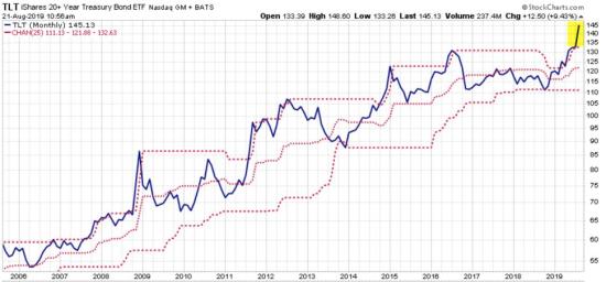
…and speaking of Technical Analysis, Long Term U.S. Treasury Bond ETF TLT has been in a volatility expansion, on the upside. Demand has driven its price momentum up to levels historically seen during larger stock market declines. The price is now outside the upper price channel. You can probably observe what it typically does afterward.
technical analysis of TLT $TLT trend following

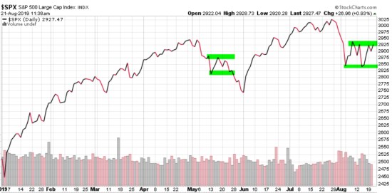
Technical Analysis of the S&P 500 index price trend: it looks to me like we’re about to observe a breakout in one direction or the other. The last time, in May, the breakout was to the downside. This time may be different. See the first image above for risk disclosure of what may go wrong — or at least who may be blamed for it 🙂
technical analysis of the stock market spx

Technical Analysis of VIX: the volatility expansion has now contracted from 25 to 15. So, the options market now expects the range to be within 15% instead of 25%.

We’ll see if vol expectations continue to drift down, or spike back up.

Ps. I didn’t provide any evidence of my political beliefs. If anyone took anything from the above as a sway one way of the other, they are joking themselves as I am joking with them. I focus on the facts. We can’t blame any single thing or any one person on the direction of stock market trends and if anyone does so, they are joking themselves.

We can say the same for calling Technical analysis Quantitative analysis, believing by changing the word, it means something different.

It doesn’t.

I say believe and do whatever creates asymmetric investment returns for you.

But as Larry the Cable Guy says:

Now that’s funny right there; I don’t care who you are!


Mike Shell is the Founder and Chief Investment Officer of Shell Capital Management, LLC, and the portfolio manager of ASYMMETRY® Global Tactical.

Mike Shell and Shell Capital Management, LLC is a registered investment advisor and provides investment advice and portfolio management exclusively to clients with a signed and executed investment management agreement. The observations shared on this website are for general information only and should not be construed as advice to buy or sell any security. Securities reflected are not intended to represent any client holdings or any recommendations made by the firm. Investing involves risk, including the potential loss of principal an investor must be willing to bear. Past performance is no guarantee of future results. All information and data is deemed reliable, but is not guaranteed and should be independently verified. The presence of this website on the Internet shall in no direct or indirect way raise an implication that Shell Capital Management, LLC is offering to sell or soliciting to sell advisory services to residents of any state in which the firm is not registered as an investment advisor. Use of this website is subject to its terms and conditions.

Stock Market Decline is Broad

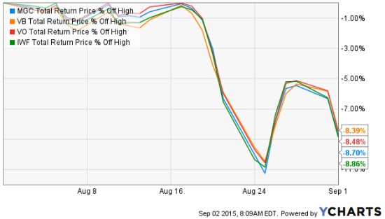
We typically expect to see small company stocks decline first and decline the most. The theory is that smaller companies, especially micro companies, are more risky so their value may disappear faster.  Below, we view the recent price trends of four market capitalization indexes: micro, small, mid, and mega. We’ll use the following index ETFs.

Vanguard ETFs small mid large micro cap

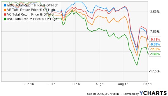
Since we are focused on the downside move, we’ll only observe the % off high chart. This shows what percentage the index ETF had declined off its recent highest price (the drawdown). We’ll also observe different look-back periods.

We first look back 3 months, which captures the full extent of the biggest loser: as expected, the micro cap index. The iShares Micro-Cap ETF (IWC: Green Line) seeks to track the investment results of an index composed of micro-capitalization U.S. equities. Over the past 3 months (or anytime frame we look) it is -13% below its prior high. The second largest decline is indeed the small cap index. The Vanguard Small-Cap ETF (VB: Orange Line) seeks to track the performance of the CRSP US Small Cap Index, which measures the investment return of small-capitalization stocks. The small cap index has declined -11.5%. The Vanguard Mega Cap ETF (MGC) seeks to track the performance of a benchmark index that measures the investment return of the largest-capitalization stocks in the United States and has declined -9.65%. The Vanguard Mid-Cap ETF (VO) seeks to track the performance of a benchmark index that measures the investment return of mid-capitalization stocks and has declined -9.41%. So, the smaller stocks have declined a little more than larger stocks.

Small and Micro caps lead down

Source: Shell Capital Management, LLC created with http://www.ycharts.com

Many active or tactical strategies may shift from smaller to large company stocks, hoping they don’t fall as much. For example, in a declining market relative strength strategies would rotate from those that declined the most to those that didn’t. The trouble with that is they may still end up losing capital and may end up positioned in the laggards long after a low is reached. They do that even though we may often observe the smallest company stocks rebound the most off a low. Such a strategy is focused on “relative returns” rather than “absolute returns“. An absolute return strategy will instead exit falling trends early in the decline with the intention of avoiding more loss. We call that “trend following” which has the objective of “cutting your losses short”. Some trend followers may allow more losses than others. You can probably see how there is a big difference between relative strength (focusing on relative trends and relative returns)  and trend following (focusing on actual price trends and absolute returns).

So, what if we look at the these stock market indexes over just the past month instead of the three months above? The losses are the same and they are very correlated. So much for diversification. Diversification across many different stocks, even difference sizes, doesn’t seem to help in declining markets on a short-term basis. These indexes combined represent thousands of stocks; micro, small, medium, and large. All of them declined over -11%, rebounded together, and are trending down together again.

stock market returns august 2015

Source: Shell Capital Management, LLC created with http://www.ycharts.com

If a portfolio manager is trying to “beat the market” index, he or she may focus on relative strength or even relative value (buy the largest loser) as they are hoping for relative returns compared to an index. But a portfolio manager who is focused on absolute returns may pay more attention to the actual downside loss and therefore focuses on the actual direction of the price trend itself. And, a key part is predefining risk with exits.

You can probably see how different investment managers do different things based on our objectives. We have to decide what we want, and focus on tactics for getting that.

Asymmetric Returns of World Markets YTD

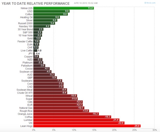
As of today, global stock, bond, commodity markets are generating asymmetric returns year to date. The graph below illustrates the asymmetry is negative for those who need these markets to go “up”.

Asymmetric Returns of World Markets 2015-04-10_10-52-47

source: http://finviz.com


Asymmetric Sector Exposure in Stock Indexes

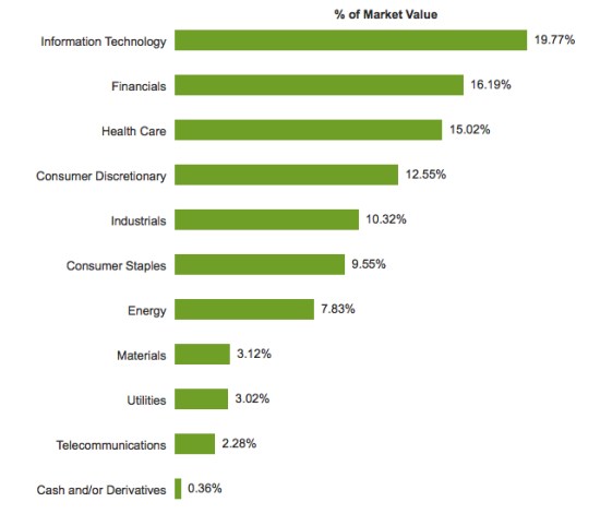
When you look at the table below and see the sector exposure percents, what do you observe? Do these allocations make sense?

asymmetric sector ETF expsoure S&P 500 2015-03-24_16-39-11

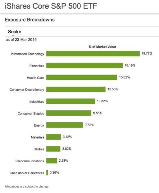
That is the sector exposure of the S&P 500 stock index: I used the iShares S&P 500 ETF for a real-world proxy. The source of each image is the index website on iShares, which you can see by clicking on the name of the index ETF.

  • Asymmetric is an imbalance. That is, more of one thing, less of another.
  • A sector is a specific industry, like Energy (Exxon Mobil) or Telecom (Verizon).
  • Exposure is the amount of the position size or allocation.

Most of the sector exposure in the S&P 500 large company stock index is Technology, Financials, Healthcare, and Consumer Discretionary. Consumer Staples, Energy, Materials, Utilities, and Telecommunications have less than 10% exposure each. Exposure to Materials, Utilities, and Telecommunications are almost non-existent. Combined, those three sectors are less than 10% of the index. Industrial has 10% exposure by itself.  But this index is 500 large companies, what about mid size and small companies?

asymmetric sector expsoure S&P 500 2015-03-24_16-39-11

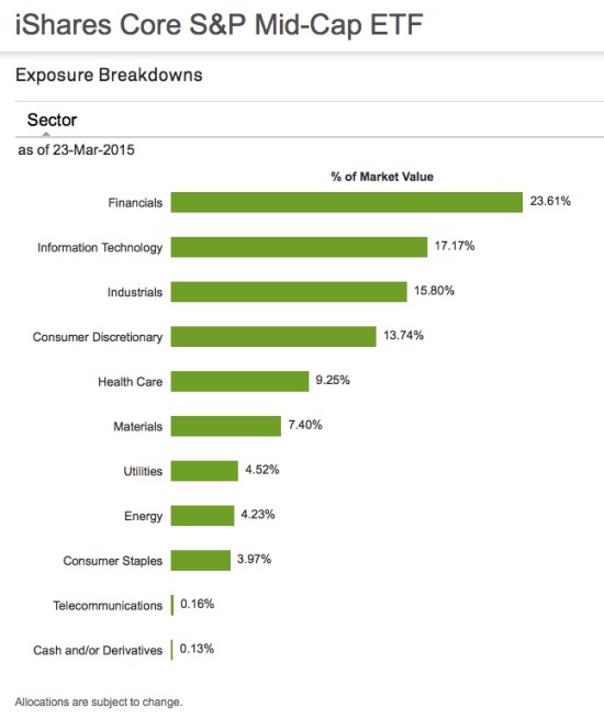
Below is the iShares Core S&P Mid-Cap ETF. Most of the sector exposure in the S&P Mid size stock index is Technology, Financials, Industrial. Healthcare, and Consumer Discretionary. Consumer Staples, Energy, Materials, Utilities, and Telecommunications have less than 10% exposure each. Exposure to Materials, Utilities, and Telecommunications are almost non-existent.

asymmetric sector exposure  S&P Mid-Cap ETF

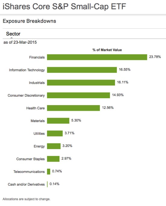
We see this same asymmetric sector exposure theme repeat in the iShares S&P Small Cap index. Half of the sectors are make up most of the exposure, the other very little.

asymmetric sector exposure S&P small cap

This is just another asymmetric observation… the next time you hear someone speak of the return of a stock index, consider they are really speaking about the return profile of certain sectors. And, these sector weightings may change over time.

US Government Bonds Rise on Fed Rate Outlook?

I saw the following headline this morning:

US Government Bonds Rise on Fed Rate Outlook

Wall Street Journal –

“U.S. government bonds strengthened on Monday after posing the biggest price rally in more than three months last week, as investors expect the Federal Reserve to take its time in raising interest rates.”

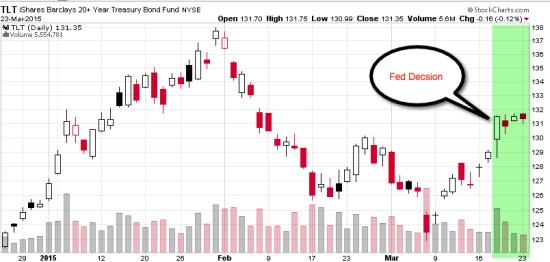
My focus is on directional price trends, not the news. I focus on what is actually happening, not what people think will happen. Below I drew a 3 month price chart of the 20+ Year Treasury Bond ETF (TLT), I highlighted in green the time period since the Fed decision last week. You may agree that most of price action and directional trend changes happened before that date. In fact, the long-term bond index declined nearly 2 months before the decision, increased a few weeks prior, and has since drifted what I call “sideways”.

fed decision impact on bonds
Charts created with http://www.stockcharts.com

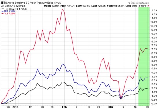
To be sure, in the next chart I included an analog chart including the shorter durations of maturity. iShares 3-7 Year Treasury Bond ETF (IEI) and iShares 7-10 Year Treasury Bond ETF (IEF). Maybe there is some overreaction and under-reaction going on before the big “news”, if anything.

Government bonds Fed decision reaction
Do you still think the Fed news was “new information“?

Trends, Countertrends, in the U.S. Dollar, Gold, Currencies

Trend is a direction that something is moving, developing, evolving, or changing. A trend is a directional drift, one way or another. When I speak of price trends, the directional drift of a price trend can be up, down, or sideways.

Trends trend to continue and are even more likely to continue than to reverse, because of inertia. Inertia is the resistance to change, including a resistance to change in direction. It’s an important physics concept to understand to understand price trends because inertia relates to momentum and velocity. A directional price trend that continues, or doesn’t change or reverse, has inertia. To understand directional price trends, we necessarily need to understand how a trend in motion is affected by external forces. For example, if a price trend is up and continues even with negative external news, in inertia or momentum is even more significant. Inertia is the amount of resistance to change in velocity. We can say that a directional price trend will continue moving at its current velocity until some force causes its speed or direction to change. A directional trend follower, then, wants keep exposure to that trend until its speed or direction does change. When a change happens, we call it a countertrend. A countertrend is a move against the prior or prevailing trend. A countertrend strategy tries to profit from a trend reversal in a directional trend that has moved to such a magnitude it comes more likely to reverse, at least briefly, than to continent. Even the best long-term trends have smaller reversals along the way, so countertrend systems try to profit from the shorter time frame oscillations.

“The one fact pertaining to all conditions is that they will change.”

                                    —Charles Dow, 1900

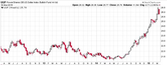
One significant global macro trend I noticed that did show some “change” yesterday is the U.S. Dollar. The U.S. Dollar has been in a smooth drift up for nearly a year. I use the PowerShares DB US Dollar Index Bullish (UUP). Below, I start with a weekly chart showing a few years so you can see it was non-trending up until last summer. Clearly, the U.S. Dollar has been trending strongly since.

u.s. dollar longer trend UPP

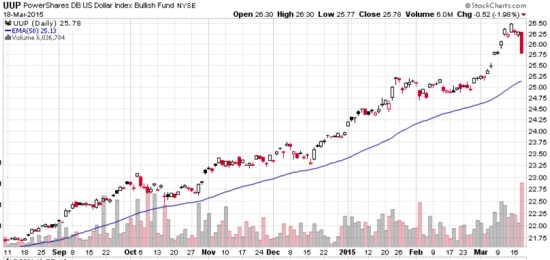
Next, we zoom in for a closer look. The the PowerShares DB US Dollar Index Bullish (UUP) was down about -2% yesterday after the Fed Decision. Notice that I included a 50 day moving average, just to smooth out the price data to help illustrate its path. One day isn’t nearly enough to change a trend, but that one day red bar is greater in magnitude and had heavy volume. On the one hand, it could be the emotional reaction to non trend following traders. On the other, we’ll see over time if that markets a real change that becomes a reversal of this fine trend. The U.S. Dollar may move right back up and resume it’s trend…

U.S. Dollar Trend 2015-03-19_08-21-35

chart source for the following charts: http://www.stockcharts.com

I am using actual ETFs only to illustrate their trends. One unique note about  PowerShares DB US Dollar Index Bullish Fund (Symbol: UUP) is the tax implications for currency limited partnership ETFs are subject to a 60 percent/40 percent blend, regardless of how long the shares are held. They also report on a K-1 instead of a 1099.

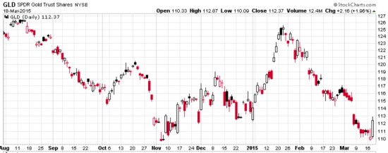
Why does the direction of the U.S. Dollar matter? It drives other markets. Understanding how global markets interact is an edge in global tactical trading. Below is a chart of Gold. I used the SPDR Gold Trust ETF as a proxy. Gold tends to trade the opposite of the U.S. Dollar.

gold trend 2015-03-19_08-22-41

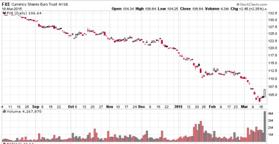
When the U.S. Dollar is trending up, it also has an inverse correlation to foreign currencies priced in dollars. Below is the CurrencyShares Euro ETF.

Euro currency trend 2015-03-19_08-23-03

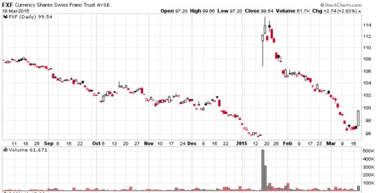
Foreign currencies can have some risk. In January, the Swiss Franc gaped up sharply, but has since drifted back to where it was. Maybe that was an over-reaction? Markets aren’t so efficient. Below is a chart of the CurrencyShares Swiss Franc to illustrate its trend and countertrend moves.

swiss franc trend 2015-03-19_08-23-23

None of this is a suggestion to buy or sell any of these, just an observation about directional trends, how they interact with each other, and countertrend moves (whether short term or long term). Clearly, there are trends…

To see how tactical decisions and understand how markets interacts results in my real performance, visit : ASYMMETRY® Managed Accounts

This is When MPT and VaR Get Asset Allocation and Risk Measurement Wrong

This is When MPT and VaR Get Asset Allocation and Risk Measurement Wrong

I was talking to an investment analyst at an investment advisory firm about my ASYMMETRY® Global Tactical and he asked me what the standard deviation was for the portfolio. I thought I would share with you how the industry gets “asset allocation” and risk measurement and management wrong.

Most people have poor results over a full market cycle that includes both rising and falling price trends, like global bull and bear markets, recessions, and expansions. Quantitative Analysis of Investor Behavior, SPIVA, Morningstar and many academic papers have provided empirical evidence that most investors (including professionals) have poor results over the long periods. For example, they may earn gains in rising conditions but lose their gains when prices decline. I believe one reason is they get too aggressive at peaks and then sell in panic after losses get too large, rather than properly predefine and manage risk.

You may consider, then, to have good results over a long period, I necessarily have to believe and do things very differently than most people.

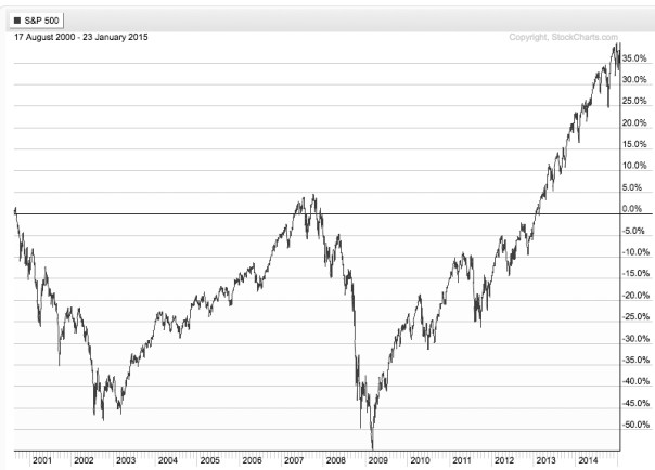
On the “risk measurement” topic, I will share with you a very important concept that is absolutely essential for truly actively controlling loss. The worst drawdown “is” the only risk metric that really matters. The risk is not the loss itself. Once we have a loss, it’s a loss. It’s beyond the realm of risk. Since risk is the possibility of a loss, how often it has happened in the past and the magnitude of the historical loss is the expectation. Beyond that, we must assume it could be even worse some day. For example, if the S&P 500 stock index price decline was -56% from 2007 to 2009, then we should expect -56% is the loss potential (or worse). When something has happened before, it suggests it is possible again, and we may have not yet observed the worst decline in the past that we will see in the future.

The use of standard deviation is one of the very serious flaws of investors attempting to measure, direct, and control risk. The problem with standard deviation is that the equation was intentionally created to simplify data. The way it is used draws a straight line through a group of data points, which necessarily ignores how far the data actually spreads out. That is, the standard deviation is intended to measure how far the data spreads out, but it actually fails to absolutely highlight the true high point and low point. Instead, it’s more of an average of those points. However, for risk management, it’s the worst-case loss that we really need to focus on. I believe in order to direct and control risk, I must focus on “how bad can it really get”. Not just “on average” how bad it can get. The risk in any investment position is at least how much it has declined in the past. And realizing it could be even worse some day. Standard deviation fails to reflect that in the way it is used.

Consider that as prices trend up for years, investors become more and more complacent. As investors become complacent, they also become less indecisive as they believe the recent past upward trend will continue, making them feel more confident. On the other hand, when investors feel unsure about the future, their fear and indecisiveness is reflected as volatility as the price swings up and down more. We are always unsure about the future, but investors feel more confident the past will continue after trends have been rising and volatility gets lower and lower. That is what the peak of a market looks like. As it turns out, that’s just when asset allocation models like Modern Portfolio Theory (MPT) and portfolio risk measures like Value at Risk (VaR) tell them to invest more in that market – right as it reaches its peak. They invest more, complacently, because their allocation model and risk measures tell them to. An example of a period like this was October 2007 as global stock markets had been rising since 2003. At that peak, the standard deviation was low and the historical return was at its highest point, so their expected return was high and their expected risk (improperly measured as historical volatility) was low. Volatility reverses the other way at some point

What happens next is that the market eventually peaks and then begins to decline. At the lowest point of the decline, like March 2009, the global stock markets had declined over -50%. My expertise is directional price trends and volatility so I can tell you from empirical observation that prices drift up slowly, but crash down quickly. The below chart of the S&P 500 is an example of this asymmetric risk.

stock index asymmetric distribution and losses

At the lowest point after prices had fallen over -50%, in March 2009, the standard deviation was dramatically higher than it was in 2007 after prices had been drifting up. At the lowest point, volatility is very high and past return is very low, telling MPT and VaR to invest less in that asset. This is a form of volatility targeting: investing more at lower levels or historical volatility and less at higher levels.

In the 2007 – 2009 decline in global markets, you may recall some advisors calling it a “6 sigma event”. That’s because the market index losses were much larger than predicted by a standard deviation. For example, if an advisors growth allocation had an average return of 10% in 2007 based on its past returns looking back from the peak and a standard deviation of 12% expected volatility, they only expected the portfolio would decline -26% (3 standard deviations) within a 99.7% confidence level – but the allocation actually lost -40 or -50%. Even if that advisor properly informed his or her client the allocation could decline -26% worse case and the client provided informed consent and acceptance of that risk, their loss was likely much greater than their risk tolerance. When they reach their risk tolerance, they “tap out”. Once they tap out, when do they ever get back in? do they feel better after it falls another -20%? or after it rises 20%? There is no good answer. I want to avoid that situation. I prefer to reduce my exposure to loss in well advance.

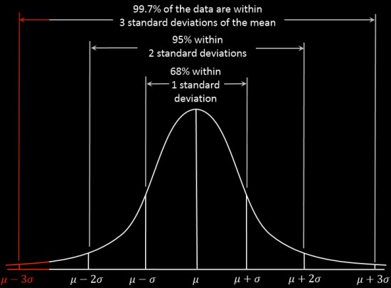
You can see in the chart below, 3 standard deviations is supposed to capture 99.7% of all of the data if the data is a normal distribution. The trouble is, market returns are not a normal distribution. Instead, stock market gains and losses present an asymmetrical return distribution. Market returns experience much larger gains and losses than expected from a normal distribution – the outliers are critical. However, those outliers don’t occur very often: historically it’s maybe every 4 or 5 years, so people have time to forget about the last one and become complacent.

symmetry normal distribution bell curve black

Source: http://en.wikipedia.org/wiki/68%E2%80%9395%E2%80%9399.7_rule

My friends, this is where traditional asset allocation like Modern Portfolio Theory (MPT) and risk measures like Value at Risk (VaR) get it wrong.

These methods are the most widely believed and used . You can probably see why most investors do poorly and only a very few do well – an anomaly.

I can tell you that I measure risk by how much I can lose and I control my risk by predefining my absolute risk at the point of entry and my exit point evolves as the positions are held. That is an absolute price point, not some equation that intentionally ignores the outlier losses.

As the stock indexes have now been overall trending up for 5 years and 9 months, the trend is getting aged. In fact, according to my friend Ed Easterling at Crestmont Research, at around 27 times EPS the stock index seems to be in the range of overvalued. In his latest report, he says:

“The stock market surged over the past quarter, adding to gains during 2014 that far exceed underlying economic growth. As a result, normalized P/E increased to 27.2—well above the levels justified by low inflation and interest rates. The current status is approaching “significantly overvalued.”

At the same time, we shouldn’t be surprised to eventually see rising interest rates drive down bond values at some point. It seems from this starting point that simply allocating to stocks and bonds doesn’t have an attractive expected return.

I believe a different strategy is needed, especially form this point forward.

In ASYMMETRY® Global Tactical, I actively manage risk and shift between markets to find profitable directional price trends rather than just allocate to them.


Mike Shell is the Founder and Chief Investment Officer of Shell Capital Management, LLC, and the portfolio manager of ASYMMETRY® Global Tactical.

The observations shared on this website are for general information only and are not specific advice, research, or buy or sell recommendations for any individual. Investing involves risk including the potential loss of principal an investor must be willing to bear. Past performance is no guarantee of future results. The presence of this website on the Internet shall in no direct or indirect way raise an implication that Shell Capital Management, LLC is offering to sell or soliciting to sell advisory services to residents of any state in which the firm is not registered as an investment advisor. Use of this website is subject to its terms and conditions.
 

Small vs. Large Stocks: A Tale of Two Markets (Continued)

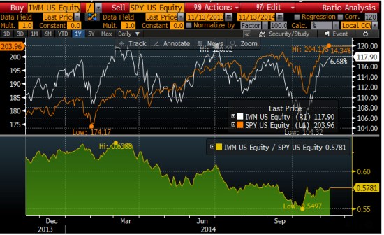
A quick follow up to my recent comments about the down trend in smaller company stocks in Playing with Relative Strength and Stock Market Peak? A Tale of Two Markets below is a chart and a few observations:

Rusell 2000 Small Caps vs S&P 500 large caps

Source: Bloomberg/KCG

A few observations of the trend direction, momentum, and relative strength.

  • The S&P 500 index (the orange line) of large company stocks has been  in a rising trend of higher highs and higher lows (though that will not continue forever).
  • The white line is the Russell 2000 small company index has been in a downtrend of lower highs and lower lows, though just recently you may observe in the price chart that it is at least slightly higher than its August high. But it remains below the prior two peaks over the past year. From the time frame in the chart, we could also consider it a “non-trending” and volatile period, but its the lower highs make it a downtrend.
  • The green chart at the bottom shows the relative strength between S&P 500 index of large company stocks and the Russell 2000 small company index. Clearly, it hasn’t taken all year to figure out which was trending up and the stronger trend.
  • Such periods take different tactical trading skills to be able to shift profitability. When markets get choppy, you find out who really knows what they’re doing and has an edge. I shared this changing trend back in May in Stock Market Peak? A Tale of Two Markets.

If you are unsure about the relevance of the big picture regarding these things, read Playing with Relative Strength and Stock Market Trend: reverse back down or continuation? and Stock Market Peak? A Tale of Two Markets.


Fun with Weather Graphs: A Quant View of Knoxville Relative to Tampa

I recently compared the climate differences between two places I call home: Knoxville, Tennessee and Tampa, Florida. They have very different climates, Knoxville is in the Tennessee mountains, the Tampa Bay/Clearwater/St. Pete area is home of the best beaches in America.  Some of us consider the two the best of both worlds. What you believe depends on your own experience. Knoxville is one of the gateways to the Great Smoky Mountains National Park, the most visited national park in America. It had about 10 million visitors in 2013, which was double the Grand Canyon, the second most visited. The two cities have very different climates in the summer and winter months. We think of Tampa, Florida as hot and sunny. Knoxville is cooler in the summer, chilly in the winter. But that’s just my opinion and description. If we really want to understand the absolute level of temperature, humidity, and sunshine, and relative differences we can apply some quantitative methods and draw some visual graphs between them. Here you will see how I see and understand how I make decisions and draw distinctions. For those who otherwise have difficultly understanding data and graphs, you may find it more interesting to apply the same concepts to the weather.  I’ll share with you my study of Knoxville vs. Tampa weather which I think is a good example of applying historical data to understand what to expect. To do this weather comparison, I used this tool with data from the NOAA Comparative Climate Data.

Summer in Knoxville, Winter in Tampa?

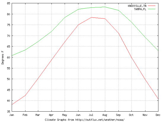
Initially, we can compare the average temperature between Knoxville and Tampa to get a quick visual. We can see some positive asymmetry between the winter and summer months. The average temperature in January is in the 60’s in Tampa and only the 30’s in Knoxville: a 30 degree spread. Yet, the average summer months is only a 10 degree spread. I call that positive asymmetry, because we don’t want it too hot in the summer and we don’t want it too cool in the winter. Tampa has the better tradeoff. But, the flaw of averages is that the actual high and low range can be much wider than we realize, so can gain a better understanding by looking specifically at the highs and lows.

AVERAGE TEMP

average temperature knoxville tampa


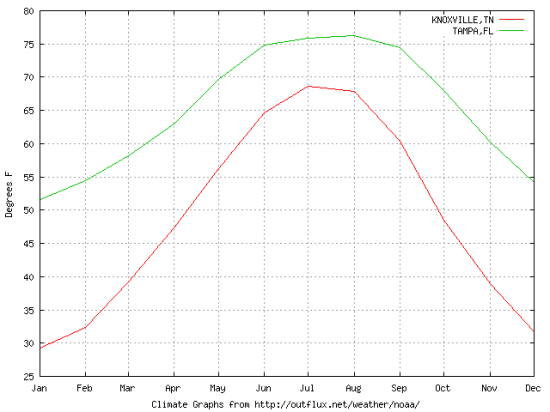
Although Knoxville is in the south, it still gets cold in the winter months. If we wanted a “winter home” to avoid those cold winter months, we would first focus on the average low temperature. That is, “how cold does it get”? Comparing the lows allows us to understand how cold it gets. As we see in the chart below, January and February are the coldest months in Knoxville when the low is around freezing. On the other hand, in Tampa the average low is above 50. 50 is chilly, not really cold. Notice the other extreme on the chart is the peak, when the average low in Tampa is over 70 during starting in June through September. We could say that that weather in Knoxville is more volatile throughout the year since it has a wider range of temperatures. We can see the visually by how quickly the data spreads out or how steep it is between the summer months and colder months. Clearly, the average lows of Tampa are more comfortable if you enjoy the outdoors.

AVERAGE LOW

average low


What about summer?

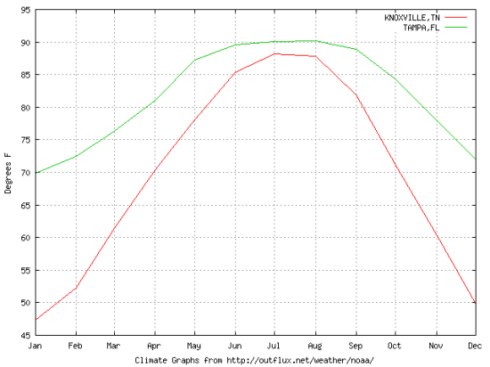
We know that the further south we go, the hotter the summers we can expect. To see that visually, we can graph the average high temperatures. In Tampa, the average high is above 70 year around. The cold months in Knoxville have an average high around or below 50. When we consider the average low in Knoxville is in the 30’s and average high is the 50’s, that’s a material difference from an average low in Tampa in the 50’s and average high in the comfortable 70’s. In fact, you may observe the average low in Tampa is the average high in Knoxville.

But what about too much heat? While the average high in Knoxville is in July and just short of 90, Tampa stays as hot as Knoxville hottest month from May up to October. For some, Tampa may be too hot in the summer. But humidity has a lot of do with how hot it feels, we’ll get to that.

AVERAGE HIGH

average high


What about extreme cold?

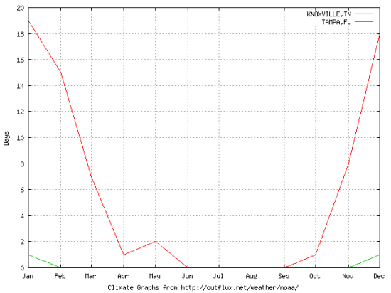
When we analyze data, we want to look at it in different ways to carve out the things we want (warm weather) and carve away the things we don’t (cold and hot weather). Below we graph for a visual to see the average days below freezing (32F). Clearly, Knoxville experiences some freezing days that are rare in Tampa, Florida. Some of you are probably laughing at my calling below 32F “extreme cold”, thinking it should be instead below zero. What you consider extreme depends on your own judgment and experience.

 AVERAGE DAYS BELOW 32F

average days below 30 degrees knoxville tampa

What about extreme heat?

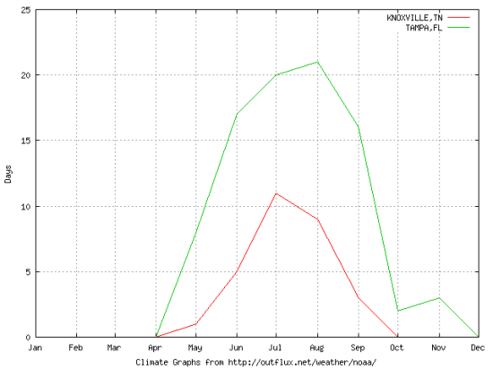
When we state an extreme, we have to define what we mean by extreme quantitatively. I used 90F to define an extremely hot day. As we see below, while Knoxville has many more days below freezing in the winter, Tampa has many more days of extreme heat in the summer. We are starting to discover when we want to be in Knoxville, Tennessee and when we may want to be in Tampa, Florida. As with investment management, timing is everything.

AVERAGE DAYS ABOVE 90F

average days over 90 degrees tampa florida knoxville tennessee

What about Precipitation?

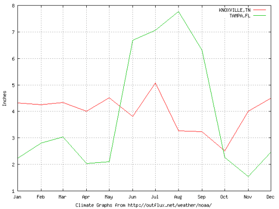
It doesn’t matter if the weather feels great if it’s raining all the time. Tampa experiences a lot of rainfall in inches starting in May through September. Knoxville rainfall is actually a little less in the summer months. So, we could describe Tampa as hot wet summers and Knoxville as warm dry summers.

AVERAGE PRECIPITATION

AVERAGE RAIN PRECIPITATION KNOXVILLE TAMPA


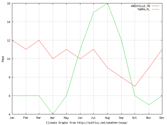
A little rain is one thing and may not be significant. What if we define a “significant rain” as greater than 0.10 inches? The stand out is that Tampa has “significant rain” in the summer months and little in the winter.

AVERAGE DAYS OF PRECIPITATION LESS GREATER THAN 0.10 INCHES

average rain days over tenth of inch in tampa knoxville


What about Humidity?

If you’ve ever experienced a place like Vail, Colorado in the winter were you can sit outside for lunch in the snow without a coat on when it’s 32F, you’ll have a unique understanding of humidity. We can say the same for south Florida in July. Humidity is the amount of water vapor in the air. Humidity may take more explanation to better understand. According to Wikipedia:

Higher humidity reduces the effectiveness of sweating in cooling the body by reducing the rate of evaporation of moisture from the skin. This effect is calculated in a heat index table or humidex, used during summer weather.

There are three main measurements of humidity: absolute, relative and specific. Absolute humidity is the water content of air. Relative humidity, expressed as a percent, measures the current absolute humidity relative to the maximum for that temperature. Specific humidity is a ratio of the water vapor content of the mixture to the total air content on a mass basis.

Relative humidity is an important metric used in weather forecasts and reports, as it is an indicator of the likelihood of precipitation, dew, or fog. In hot summer weather, a rise in relative humidity increases the apparent temperature to humans (and other animals) by hindering the evaporation of perspiration from the skin. For example, according to the Heat Index, a relative humidity of 75% at 80.0°F (26.7°C) would feel like 83.6°F ±1.3 °F (28.7°C ±0.7 °C) at ~44% relative humidity.

The temperature alone isn’t the full measure of how hot and uncomfortable the climate can be. We can break down humidity into morning and afternoon. Morning humidity in Knoxville is highest in the winter months, which leads to a cold, wet feeling winter. Morning humidity in Tampa is highest in the summer, making hot feel even hotter.

AVERAGE MORNING HUMIDITY

average morning humidity knoxville tampa


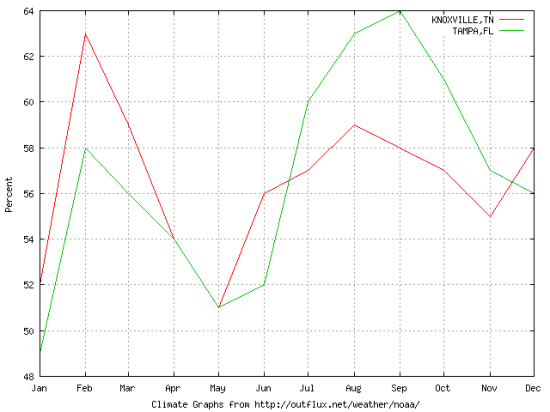
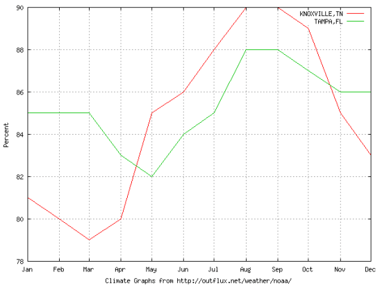
As we see below, afternoon humidity is much higher in Knoxville during the summer months.Tampa stays above 82% humidity on average. By now you have probably began to spot directional trends in the data as well as mean reversion. For example, in the chart below the red line (Knoxville) trends upward sharply from March to August. Then it reverses back down to retrace about half the prior gain. I see the same patterns and trends in global markets, though they are more difficult based more on social science than the science of climate and seasons. Yet, there are seasonal patters in global markets, too, such as “sell in May and go away” and “January Effect”. But unlike weather changes, they seasonal changes in the stock market aren’t as sure as the transition from summer to fall to winter to spring to summer again in Tennessee.

AVERAGE AFTERNOON HUMIDITY

average afternoon humidity knoxville tampa

Tampa has a Breeze

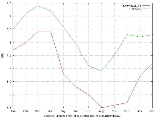
Below we see the average wind speed. Tampa has a breeze to help cool us down compared to Knoxville.

average wind speed tampa florida knoxville tennessee

What about Sunshine?

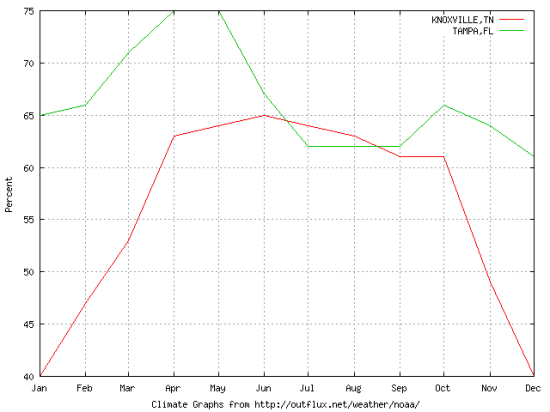
Warm dry weather is nice, but what about sunshine? Below we see why they say “Sunny Florida”. You may notice that Tampa is more sunny in the winter months then even the summer months. Knoxville has a greater possibility of sunshine March through October with a sharp downtrend on both ends.

AVERAGE SUNSHINE POSSIBLE

AVERAGE SUNSHINE POSSIBLE TAMPA KNOXVILLE

What about Cloudy Days?

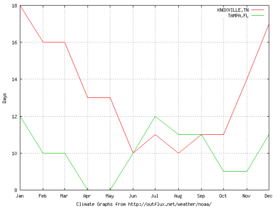
If you live in the north, you are familiar not only with cold wet winters, but cloudy grey skies. The outliear that stands out on this graph is that Knoxville is cloudy half of the days of each month in the winter. Tampa, on the other hand, has few cloudy days throughout the year, but its highest is the July. You may have noticed some climate patterns between Tampa and Knoxville are negatively correlated. That is, Knoxville tends to be cloudy in January and least cloudy in July and Tampa is nearly the opposite.

AVERAGE DAYS CLOUDY

average cloudy days knoxville tampa

In the late 1990’s I remember listening to Steven Covey audiobook of “7 Habits of Highly Effective People” when he would say: “proactive people carry weather with them”. That is an example of Projection makes perception: seek not to change the weather, but to change your mind about the weather. That may work for some of us for many years, but eventually we may instead decide to “rotate instead of allocate”. That is, we may decide a warm sunny place like Tampa, Florida is a great place when its cold, wet, and cloudy in a place like Knoxville. Though, Knoxville may be better to spend the summer months with its more mild summer than the hot humid wet Tampa summer.

You can “carry weather with you” by perceiving it how you want, or you can carry (rotate) yourself to the weather you prefer. You can probably see how this quantitative data study helps visualize the absolute climate ranges and relative differences to make the decision with a greater understanding of what to expect.